Color-based Skin Tracking
Under Varying Illumination:
Experiments

Color-based Skin Tracking
Under Varying Illumination: |
|
 |
 |
 |
 |
 |
 |
 |
 |
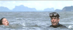 |
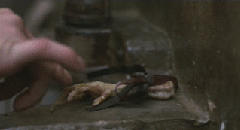
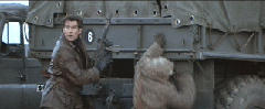
All experimental sequences were hand-labeled to provide the ground truth data for algorithm performance verification. Every fifth frame of the sequences was labeled. For each labeled frame, the human operator created one binary image mask for skin regions and one for non-skin regions (background). Boundaries between skin regions and background, as well as regions that had no clearly distinguishable membership in either class were not included in the masks and are considered {\em don't care} regions. The segmentation of these regions was not counted during the experimentation or evaluation of the system. The figure below shows one example frame and its ground-truth labeling.
(a) |
(b) |
(c) |
(d) |
For comparison, we measured the classification performance of a standard static histogram segmentation approach on the same data set. The static histogram approach implemented used the same prior histograms and threshold as our adaptive system (see the technical report for more details). The same binary image processing operations of connected component analysis, size filtering, and hole filtering were performed to achieve a fair comparison.
| Classification Performance | |||||||
| Sequence Info | Static | Dynamic | |||||
| # | \char93 frames | skin | bg | Det[C] | skin | bg | Det[C] |
| 1 | 71 | 70.2 | 97.5 | 0.67 | 72.2 | 96.9 | 0.69 |
| 2 | 349 | 64.3 | 100 | 0.64 | 74.8 | 100 | 0.75 |
| 3 | 52 | 92.9 | 98.5 | 0.91 | 96.4 | 97.8 | 0.94 |
| 4 | 99 | 46.2 | 100 | 0.46 | 56.7 | 99.9 | 0.57 |
| 5 | 71 | 90.2 | 100 | 0.90 | 96.9 | 100 | 0.97 |
| 6 | 71 | 96.3 | 100 | 0.96 | 97.5 | 100 | 0.98 |
| 7 | 74 | 90.7 | 95.4 | 0.86 | 91.6 | 94.0 | 0.86 |
| 8 | 119 | 15.1 | 100 | 0.15 | 38.3 | 100 | 0.38 |
| 9 | 71 | 85.9 | 99.5 | 0.85 | 89.8 | 99.5 | 0.89 |
| 10 | 71 | 77.1 | 91.6 | 0.69 | 77.8 | 89.8 | 0.68 |
| 11 | 109 | 92.4 | 99.7 | 0.92 | 94.5 | 99.5 | 0.94 |
| 12 | 49 | 43.1 | 100 | 0.43 | 69.2 | 100 | 0.69 |
| 13 | 74 | 96.9 | 99.9 | 0.97 | 97.6 | 99.9 | 0.97 |
| 14 | 74 | 97.8 | 100 | 0.98 | 98.3 | 100 | 0.98 |
| 15 | 90 | 87.3 | 100 | 0.87 | 86.5 | 100 | 0.87 |
| 16 | 75 | 74.7 | 100 | 0.75 | 84.3 | 100 | 0.84 |
| 17 | 72 | 98.6 | 98.8 | 0.97 | 98.6 | 98.8 | 0.97 |
| 18 | 71 | 81.5 | 99.8 | 0.81 | 88.0 | 100 | 0.88 |
| 19 | 71 | 36.3 | 100 | 0.36 | 37.6 | 100 | 0.38 |
| 20 | 71 | 93.2 | 37.5 | 0.31 | 97.1 | 36.6 | 0.34 |
| 21 | 232 | 83.6 | 100 | 0.84 | 83.4 | 100 | 0.83 |
| Average | 76.9 | 96.1 | 0.73 | 82.2 | 95.8 | 0.78 | |
The performance results are outlined in the table shown above. Three
performance measures were computed: correct classification of skin pixels,
correct classification of background pixels, and the determinant of the
confusion matrix
The five sequences that failed to perform better, had an insignificant performance loss. In all five failure cases, the system performed no worse than 1%. This performance degradation was due to skin-like color patches appearing in the background of initial frames of a sequence. Recall that these initial frames are used in in estimating the parameters of the Markov model (see technical report for more details).
Finally, we performed a set of experiments to establish system stability over time. For example, the graph in below shows system performance on the longest sequence in our test set (349 frames).
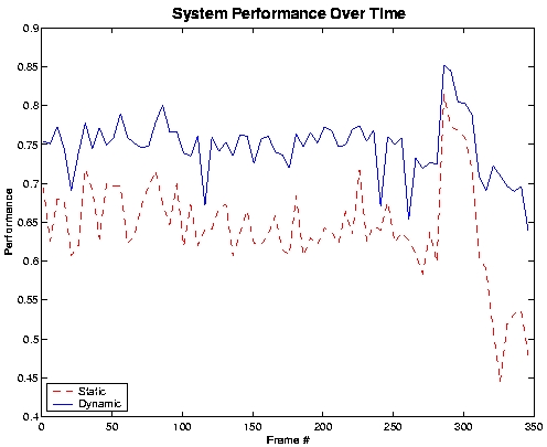
As can be seen from the graph, the dynamic approach was consistently better than the static method in classifying skin and background pixels. Not only does our system perform over 10% better for the entire sequence, it is also more stable. The standard deviation of performance for our system was measured to be 0.0375, which is almost a half of the standard deviation of 0.0630 measured for the static segmentation approach. It should be noted that the stability of our system was consistent across experiments.
Last Modified: March 14, 2000