Old version
This is the CS 111 site as it appeared on May 10, 2018.
Problem Set 7
Preliminaries
In your work on this assignment, make sure to abide by the collaboration policies of the course.
Don’t forget to use docstrings and to take whatever other steps are needed to create readable code.
If you have questions while working on this assignment, please
come to office hours, post them on Piazza, or email
cs111-staff@cs.bu.edu.
Make sure to submit your work on Apollo, following the procedures found at the end of the assignment.
Part I
due by 11:59 p.m. on Thursday, March 29, 2018
Problem 0: Reading and response
5 points; individual-only
Some of the remaining problems in this assignment will involve using 2-D lists to implement Conway’s Game of Life. This game can be seen as a form of computation–but of a very different sort than we typically encounter.
Unlike typical top-down computation, in which everything is coordinated in a centralized fashion, you’ll see that the Game of Life is a bottom-up, decentralized computation in which separate “cells” interact with only their immediate neighbors to determine what should happen next. Such an approach is more biological in nature, with results emerging from many local processes rather than a single, overarching one.
This week’s reading is an article from Josh Bongard about the forms that biologically-inspired computing have taken–and may take in the future.
After reading his article, write a short response that addresses the following question: What are the advantages and disadvantages of pursuing a strategy of evolving programs to solve problems, rather than writing them for a specific task?
Put your response in a file named ps7pr0.txt. Don’t forget that the
file you submit must be a plain-text file.
Problem 1: Working with nested loops and 2-D lists
10 points; individual-only
Put your answers for this problem in a plain-text file named
ps7pr1.txt.
-
Consider the following Python program, which uses a nested loop:
for x in [3, 4, 5]:
    for y in range(2, x):
        print(x + y)
print(x, y)
Copy the table shown below into your text file for this problem, and complete it (adding rows as needed) to show how the variables change over time and the values that are printed.
  x  | range(2, x) |  y  | value printed
----------------------------------------
  3  | [2]         |  2  | 5
     |             |     |
Hint: The lecture and lab exercises include similar traces.
-
Consider the following Python statement, which creates a two-dimensional list of integers:
twoD = [[1, 2, 3],
        [4, 5, 6],
        [7, 8, 9]]
-
Write an assignment statement that replaces the value of 6 in this 2-D list with a value of 12.
-
Write a code fragment that uses a loop to print the values in the leftmost column of the 2-D list to which
twoDrefers. Print each value on its own line.For the list above, the following values would be printed:
1
4
7
Your code should be general enough to work on any two-dimensional list named
twoDthat has at least one value in each row. -
Write a code fragment that uses one or more loops to print the values in the anti-diagonal of the list to which
twoDrefers – i.e., the values along a diagonal line from the bottom-left corner to the upper-right corner. Print each value on its own line.For the list above, the following values would be printed:
7
5
3
Your code should be general enough to work on any two-dimensional list in which the dimensions are equal – i.e., the number of rows is the same as the number of columns.
Hint: To determine the necessary pattern, make a table showing the row and column indices of each element in the anti-diagonal. What is true about each pair of indices?
For all of these tasks, you are welcome to use IDLE to write and test your code to ensure that it accomplishes the specified tasks. However, you should include your final answers in your
ps7pr1.txtfile. -
Problem 2: TT Securities
25 points; individual-only
This problem involves using loops to process a list of stock prices. You will also gain experience in writing a program that involves repeated user interactions.
The premise behind this problem is that you have been hired by an investment firm called Time Travel Securities, Inc. (also known as TT Securities or TTS). They want you to write a program that will perform a variety of tasks involving a list of stock prices.
We will discuss this application in lecture and look at an example
user-interaction loop. In ps7pr2.py, we’ve
given you some starter code that is based on the code from lecture.
Download that file, open it in IDLE, and add the code needed to
support the functionality described below.
Important
-
You may not use the built-in
sum,min, ormaxfunctions for this problem. Instead, you should use loops of your own construction to compute the necessary values. -
As usual, you should include a docstring and any other comments that might be necessary to explain your code. More generally, you should aim to make your code easy to read. For example, you should choose descriptive names for your variables. In addition, we encourage you to leave a blank line between logical parts of your function.
-
If you want to add test calls to this or any other Python file, please do so in appropriate test function like the one that we gave you at the bottom of the
ps1pr3.pystarter file for Problem Set 1. After running your Python file, you can call thetestfunction (by enteringtest()) to see the results of all of the test calls.Do not add any lines of code that belong to the global scope of the program (i.e., lines that are outside of any function).
-
These guidelines apply to this and all remaining Python code that you write for this course!
Running the program
The starter code that we’ve given you includes a function called tts() that serves as the “main” function–the one that handles the
user interactions.
To run the program, you should call this function. Run ps7pr5.py
in IDLE, which you will bring you to the Shell, and then make
the following function call:
>>> tts()
Required functionality The program should present the user with the following menu of choices:
(0) Input a new list of prices
(1) Print the current prices
(2) Find the latest price
(3) Find the average price
(4) Find the standard deviation
(5) Find the min price and its day
(6) Test a threshold
(7) Your TT investment plan
(8) Quit

Enter your choice:
Our starter code includes support for a few of these options. You will need to implement the rest of them. In particular, you should perform tasks 0-5 outlined below.
A sample run that illustrates what the behavior of the program should look like is available here.
-
Read over the starter code that we’ve given you. Make sure that you understand how the various functions work, and how they fit together.
-
Add support for option 3: finding the average price
First, write a function calledavg_pricethat takes a list of 1 or more prices and computes and returns the average price. Don’t forget that you cannot use the built-insum,min, ormaxfunctions. Instead, you should use a loop of your own construction to perform the necessary computations.Here are two examples:
>>> avg_price([10, 20, 18])
16.0
>>> print(avg_price([5, 8, 5, 3]))
5.25
Next, you should integrate this function into the overall program by doing the following:
-
Update the
display_menu()function to print the description of this menu option. -
Add code to the
tts()function to call youravg_pricefunction whenever the user chooses option 3, and to print the result that it returns. See the sample run for an example of what the output of this option should look like.Important: The printing of the result should be done in
tts(). Youravg_pricefunction should not do any printing. In general, none of the new functions that you write should do any printing. Rather, you should add code totts()to print the results in the proper format.
-
-
Add support for option 4: finding the standard deviation
Begin by writing a function calledstd_devthat takes a list of 1 or more prices and computes and returns the standard deviation of the prices. Use the following formula:
Formula for standard deviation. L is the list of prices. Lavg is the average of the prices. The capital sigma (Σ) means “sum for all positions i in the list” — in other words, for each price, compute the squared difference between that price and the average. Don’t forget that you cannot use the built-in
sum,min, ormaxfunctions. However, you can use youravg_pricefunction to compute the average, and we encourage you to do so!To compute the square root, you should use the
math.sqrt()function. Our starter code already imports themathmodule for you.Here are two examples of how the function should behave:
>>> std_dev([10, 20, 18])
4.320493798938574
>>> print(std_dev([5, 8, 5, 3]))
1.7853571071357126
Next, you should integrate this function into the overall program, taking steps similar to the ones you took above. Update
display_menu(), and add code totts()to callstd_devand to print the result thatstd_dev()returns. See the sample run for an example of what the output of this option should look like. -
Add support for option 5: finding the minimum price and its day
Write a function calledmin_daythat takes a list of 1 or more prices and computes and returns the day (i.e., the index) of the minimum price. Don’t forget that you cannot use the built-insum,min, ormaxfunctions.Here are two examples:
>>> min_day([20, 10, 18])
1
>>> print(min_day([15, 18, 12, 22, 17]))
2
Next, you should integrate this function into the overall program, taking steps similar to the ones that you took above. In printing the result,
tts()should print both the day of the minimum price and the minimum price itself. See the sample run for an example of what the output should look like. -
Add support for option 6: testing a threshold
Begin by writing a function calledany_abovethat takes a list of 1 or more prices and an integer threshold, and uses a loop to determine if there are any prices above that threshold. The function should returnTrueif there are any prices above the threshold, andFalseotherwise. For example:>>> any_above([10, 20, 15], 18) True >>> print(any_above([10, 20, 15], 25)) False
Important: Make sure that you return either the boolean literal
Trueor the boolean literalFalse. Do not include quotes around these values.Next, you should integrate this function into the overall program.
In addition to the types of steps that you’ve taken for the previous options, you will also need to get the threshold from the user. Add an
inputstatement totts()that obtains the threshold, and don’t forget to convert the string that is returned byinputto an integer. See our starter code for an example of this. -
Add support for option 7: the “time travel” investment strategy discussed in lecture
First, write a function calledfind_planthat takes a list of 2 or more prices, and that uses one or more loops to find the best days on which to buy and sell the stock whose prices are given in the list of prices. The buy and sell days that you determine should maximize the profit earned, but the sell day must be greater than the buy day. The function should return a list containing three integers:- the buy day
- the sell day
- the resulting profit
For example:
>>> find_plan([40, 10, 20, 35, 25])
[1, 3, 25]
In this case, the function returns a list that indicates that the best investment plan is to buy on day 1 and sell on day 3, which gives a profit of $25. Here’s another example:
>>> print(find_plan([5, 10, 45, 35, 3]))
[0, 2, 40]
Hint: In implementing this function, you may find it helpful to adapt the example
difffunction that we covered in lecture.Don’t forget to integrate this function into the overall program, taking similar steps to the ones that you took for the earlier options. See the sample run for an example of what the output of this option should look like.
Problem 3: Functions for 2-D lists
15 points; pair-optional
This is the only problem of the assignment that you may complete with a partner. See the rules for working with a partner on pair-optional problems for details about how this type of collaboration must be structured.
This problem involves writing functions that create and manipulate two-dimensional lists of integers. Some of these functions will then be used in Part II to implement John Conway’s Game of Life.
Getting started Begin by downloading the following zip file: ps7twoD.zip
Unzip this archive, and you should find a folder named ps7twoD,
and within it several files, including ps7pr3.py. Open that file
in IDLE, and put your work for this problem in that file.
You should not move any of the files out of the ps7twoD folder.
In ps7pr3.py, we’ve given you two functions:
-
create_grid(height, width), which creates and returns a 2-D list of 0s with the specified dimensions. You worked with this function in lab. -
print_grid(grid), which prints the 2-D list specified by grid in 2-D form, with each row on its own line, and no spaces between values. This is similar to a function that you worked with in lab, but this version does not leave a space between values.Notice the statement that we use to print the value of a single cell:
print(cell, end='')
The argument
end=''indicates that Python should print nothing after the value ofcell–not a newline character (which is the default behavior), and not even a space. As a result, the values in a given row will appear right next to each other on the same line. (We can safely eliminate the spaces between values because we’re assuming that the individual cell values will each be a single digit–i.e., an integer between0and9inclusive.)
Your tasks
Important
You should continue to follow the guidelines for coding style and readability that we gave you in Problem 2.
-
To provide another example of using nested loops to manipulate a 2-D list, we’re giving you the following function, which you should copy into your
ps7pr3.pyfile:def diagonal_grid(height, width): """ creates and returns a height x width grid in which the cells on the diagonal are set to 1, and all other cells are 0. inputs: height and width are non-negative integers """ grid = create_grid(height, width) # initially all 0s for r in range(height): for c in range(width): if r == c: grid[r][c] = 1 return grid
Notice that the function first uses
create_gridto create a 2-D grid of all zeros. It then uses nested loops to set all of the cells on the diagonal–i.e., the cells whose row and column indices are the same–to1.Make sure that your copy of
diagonal_gridis working by re-running the file and trying the following:>>> grid = diagonal_grid(6, 8) >>> print_grid(grid) 10000000 01000000 00100000 00010000 00001000 00000100
-
Based on the example of
diagonal_grid, write a function Write a functionrandom_grid(height, width)that creates and returns a 2-D list ofheightrows andwidthcolumns in which the inner cells are randomly assigned either0or1, but the cells on the outer border are all0.For example (although the actual values of the inner cells will vary):
>>> grid = random_grid(10, 10)
>>> print_grid(grid)
0000000000
0100000110
0001111100
0101011110
0000111000
0010101010
0010111010
0011010110
0110001000
0000000000
Our starter code imports Python’s
randommodule, and you should use therandom.choicefunction to randomly choose the value of each cell in the grid. Use the callrandom.choice([0, 1]), which will return either a0or a1. -
As we’ve seen in lecture, copying a list variable does not actually copy the list. To see an example of this, try the following commands from the Shell:
>>> grid1 = create_grid(2, 2)
>>> grid2 = grid1      # copy grid1 into grid2
>>> print_grid(grid2)
00
00
>>> grid1[0][0] = 1
>>> print_grid(grid1)
10
00
>>> print_grid(grid2)
10
00
Note that changing
grid1also changesgrid2! That’s because the assignmentgrid2 = grid1did not copy the list represented bygrid1; it copied the reference to the list. Thus,grid1andgrid2both refer to the same list!To avoid this problem, write a function
copy(grid)that creates and returns a deep copy ofgrid–a new, separate 2-D list that has the same dimensions and cell values asgrid. Note that you cannot just perform a full slice ongrid(e.g.,grid[:]), because you would still end up with copies of the references to the rows! Instead, you should do the following:-
Use
create_gridto create a new 2-D list with the same dimensions asgrid, and assign it to an appropriately named variable. (Don’t call your new listgrid, since that is the name of the parameter!) Remember thatlen(grid)will give you the number of rows ingrid, andlen(grid[0])will give you the number of columns. -
Use nested loops to copy the individual values from the cells of
gridinto the cells of your newly created grid. -
Make sure to return the newly created grid and not the original one!
To test that your
copyfunction is working properly, try the following examples:>>> grid1 = diagonal_grid(3, 3) >>> print_grid(grid1) 100 010 001 >>> grid2 = copy(grid1) # should get a deep copy of grid1 >>> print_grid(grid2) 100 010 001 >>> grid1[0][1] = 1 >>> print_grid(grid1) # should see an extra 1 at [0][1] 110 010 001 >>> print_grid(grid2) # should not see an extra 1 100 010 001
-
-
Write a function
increment(grid)that takes an existing 2-D list of digits and increments each digit by1. If incrementing a given digit causes it to become a10(i.e., if the original digit was a9), then the new digit should “wrap around” and become a0.Important notes:
-
Unlike the other functions that you wrote for this problem, this function should not create and return a new 2-D list. Rather, it should modify the internals of the existing list.
-
Unlike the other functions that you wrote for this problem, this function should not have a
returnstatement, because it doesn’t need one! That’s because its parametergridgets a copy of the reference to the original 2-D list, and thus any changes that it makes to the internals of that list will still be visible after the function returns. -
The loops in this function need to loop over all of the cells in the grid, not just the inner cells.
For example:
>>> grid = diagonal_grid(5, 5)
>>> print_grid(grid)
10000
01000
00100
00010
00001
>>> increment(grid)
>>> print_grid(grid)
21111
12111
11211
11121
11112
>>> increment(grid)
>>> print_grid(grid)
32222
23222
22322
22232
22223
>>> grid = inner_grid(6, 4, 8)
>>> print_grid(grid)
0000
0880
0880
0880
0880
0000
>>> increment(grid)
>>> print_grid(grid)
1111
1991
1991
1991
1991
1111
>>> increment(grid)
>>> print_grid(grid)
2222
2002
2002
2002
2002
2222
Here’s another example that should help to reinforce your understanding of references:
>>> grid1 = inner_grid(5, 5, 1)
>>> print_grid(grid1)
00000
01110
01110
01110
00000
>>> grid2 = grid1
>>> grid3 = grid1[:]
>>> increment(grid1)
>>> print_grid(grid1)
11111
12221
12221
12221
11111
As you can see above, the value of
grid1has been changed. What aboutgrid2andgrid3?Before entering the statements below, see if you can predict what has happened to
grid2andgrid3. If we print them, will we see the original grid or an incremented one?Test your understanding by first entering the following:
>>> print_grid(grid2)
What do you see? Why does this make sense?
Now enter the following:
>>> print_grid(grid3)
What do you see? Why does this make sense?
(You don’t need to record your answers to these questions, but we strongly encourage you to make sure that you understand what happens here. Feel free to ask for help if you don’t understand.)
-
Part II
due by 11:59 p.m. on Sunday, April 1, 2018
Problem 4: Conway’s Game of Life
20 points; individual-only
Background
The Game of Life was invented by John Conway, who is currently a
professor of mathematics at Princeton. It’s not a game in the traditional
sense, but rather a grid of cells that changes over time according
to a few simple rules.
At a given point in time, each cell in the grid is either “alive” (represented by a value of 1) or “dead” (represented by a value of 0). The neighbors of a cell are the cells that immediately surround it in the grid.
Over time, the grid is repeatedly updated according to the following five rules:
-
All cells on the outer boundary of the grid remain fixed at 0.
-
An inner cell that has fewer than 2 alive neighbors dies (because of loneliness).
-
An inner cell that has more than 3 alive neighbors dies (because of overcrowding).
-
An inner cell that is dead and has exactly 3 alive neighbors comes to life.
-
All other cells maintain their state.
Although these rules seem simple, they give rise to complex and interesting patterns! You can find more information and a number of interesting patterns here.
Getting Started
In the ps7twoD folder that you used for Problem 3, you should find a
file named ps7pr4.py. (Note that this is not the same file that
you used for Problem 3.) Open ps7pr4.py in IDLE, and put your work for
this problem in that file. Once again, you should not move any of the
files out of the ps7twoD folder.
IMPORTANT: We have included an import statement at the top of
ps7pr4.py that imports all of the functions from your ps7pr3.py file.
Therefore, you will be able to call any of the functions that you wrote
for Problem 3.
Your tasks
-
Write a function
count_neighbors(cellr, cellc, grid)that returns the number of alive neighbors of the cell at position[cellr][cellc]in the specifiedgrid. You may assume that the indicescellrandcellcwill always represent one of the inner cells ofgrid, and thus the cell will always have eight neighbors.Here are two possible approaches that you could take to this problem:
-
first approach: You could use nested loops to compute the necessary cumulative sum. Set the ranges of the two loops so that you end up examining only the specified cell and its eight neighbors. And although these loops will end up including the specified cell, you should make sure that you don’t actually count the cell itself as one of its own neighbors!
OR
-
second approach: You could write eight separate
ifstatements to check each of the eight neighbors. If you take this approach, you will not need to use any loops.
To test your function, run the file in IDLE and enter the following from the Shell:
>>> grid1 = [[0,0,0,0,0],
             [0,0,1,0,0],
             [0,0,1,0,0],
             [0,0,1,0,0],
             [0,0,0,0,0]]
>>> print_grid(grid1)
00000
00100
00100
00100
00000
>>> count_neighbors(2, 1, grid1)   # grid1[2][1] has 3 alive neighbors
3
>>> count_neighbors(2, 2, grid1)   # we don't count the cell itself!
2
>>> count_neighbors(1, 2, grid1)
1
>>> grid2 = [[0,0,0,0,0,0],
             [0,0,1,1,0,0],
             [0,1,1,1,0,0],
             [0,0,1,0,1,0],
             [0,0,1,0,1,0],
             [0,0,0,0,0,0]]
>>> count_neighbors(2, 2, grid2)   # grid2[2][2] has 5 alive neighbors
5
>>> count_neighbors(2, 3, grid2)   # so does grid2[2][3]
5
>>> count_neighbors(3, 3, grid2)   # grid2[3][3] has 6 alive neighbors
6
-
-
Now let’s implement the rules of the Game of Life!
A given configuration of the grid in the Game of Life is known as a generation of cells. Write a function
next_gen(grid)that takes a 2-D list calledgridthat represents the current generation of cells, and that uses the rules of the Game of Life (see above) to create and return a new 2-D list representing the next generation of cells.Notes/hints:
-
Begin by creating a copy of
grid(call itnew_grid). Use one of the functions that you wrote for the previous problem! -
Limit your loops so that they never consider the outer boundary of cells. You did this already in one of the functions that you wrote for the previous problem.
-
You can use the
count_neighbors()function that you just wrote. Make sure that you count the neighbors in the current generation (grid) and not the new one (new_grid). -
When updating a cell, make sure to change the appropriate element of
new_gridand not the element ofgrid.
Testing
next_gen
Here are two patterns that you might want to take advantage of when testing your function:-
If a 3x1 line of alive cells is isolated in the center of a 5x5 grid, the line will oscillate from vertical to horizontal and back again, as shown below:
>>> grid1 = [[0,0,0,0,0],
             [0,0,1,0,0],
             [0,0,1,0,0],
             [0,0,1,0,0],
             [0,0,0,0,0]]
>>> print_grid(grid1)
00000
00100
00100
00100
00000
>>> grid2 = next_gen(grid1)
>>> print_grid(grid2)
00000
00000
01110
00000
00000
>>> grid3 = next_gen(grid2)
>>> print_grid(grid3)
00000
00100
00100
00100
00000
and so on!
-
In a 4x4 grid, if the inner cells are all alive, they should remain alive over time:
>>> grid1 = [[0,0,0,0],
             [0,1,1,0],
             [0,1,1,0],
             [0,0,0,0]]
>>> print_grid(grid1)
0000
0110
0110
0000
>>> grid2 = next_gen(grid1)
>>> print_grid(grid2)
0000
0110
0110
0000
-
Optional (but encouraged): graphical life!
We have given you functions that you can use to run a graphical
version of the Game of Life. Here’s an example of how to use it with a
random starting configuration:
>>> grid = random_grid(15, 15)
>>> show_graphics(grid)    # run the Game of Life in a graphics window
The following key presses can be used to control the simulation:
Enter(orReturn): begin/resume the simulationP: pause the simulationSpacebar: clear the gridQ: quit the simulation
When the simulation is paused, you should be able to change the state of a cell by clicking on it.
Trying other patterns
The Life Lexicon is a website that includes many examples of
interesting starting patterns. They use a different representation for
the cells in a grid: a dot . character for a dead cell and
an O character for an alive cell. For example, here is a well-known
pattern known as the Gosper glider gun:
........................O...........
......................O.O...........
............OO......OO............OO
...........O...O....OO............OO
OO........O.....O...OO..............
OO........O...O.OO....O.O...........
..........O.....O.......O...........
...........O...O....................
............OO......................
You can easily try a pattern that is specified in Life Lexicon
form by using the read_pattern function. It takes 2 inputs specifying
the amount of padding (i.e., the number of empty rows and empty columns)
that should be added around a pattern that is entered by the user. When
you call this function, it waits for you to enter a pattern in the form
found in the Life Lexicon, and it converts it into a 2-D list of
the form that our functions use.
For example:
>>> grid = read_pattern(20, 20)   # use a padding of 20 on all sides
enter the pattern:
........................O...........
......................O.O...........
............OO......OO............OO
...........O...O....OO............OO
OO........O.....O...OO..............
OO........O...O.OO....O.O...........
..........O.....O.......O...........
...........O...O....................
............OO......................
When you are prompted to enter the pattern, copy and paste it into
the Shell window and hit Enter. (It’s not a problem if you have extra
spaces at the start of some of the lines when you paste the pattern.)
You can then run the pattern graphically as indicated above.
Colors
You can also change the colors used for the alive and dead cells. For
example, to invert the default color scheme–producing something that
is more obviously Terrier-themed!–you can do the following
from the Shell before calling show_graphics:
>>> set_color(0, 'red')
>>> set_color(1, 'white')
A full list of color names is available here.
Problem 5: Images as 2-D lists
25 points; individual-only
Getting started
Begin by downloading the following zip file:
ps7image.zip
Unzip this archive, and you should find a folder named ps7image,
and within it several files, including ps7pr5.py. Open that file
in IDLE, and put your work for this problem in that file.
You should not move any of the files out of the ps7image folder.
Keeping everything together will ensure that your functions are able to
make use of the image-processing module that we’ve provided.
Among the files in the ps7image folder are several PNG images that you
can use when testing your functions. They include the following:
test.png:

spam.png:
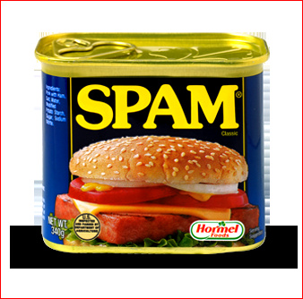
Important: Both of these images have a one-pixel border; test.png
has a blue border, and spam.png has a red one.
When you create a new image that is based on one of these images,
these borders should help you to ensure that you are transforming the
entire image.
Loading and saving pixels
At the top of ps7pr5.py, we’ve included an import statement for
the hmcpng module, which was developed at Harvey Mudd College.
This module gives you access to the following two functions that
you will need for this problem:
-
load_pixels(filename), which takes as input a stringfilenamethat specifies the name of a PNG image file, and that returns a 2-D list containing the pixels for that image -
save_pixels(pixels, filename), which takes a 2-D listpixelscontaining the pixels for an image and saves the corresponding PNG image to disk using the specifiedfilename(a string).
In addition, we’ve given you three other functions:
-
create_uniform_image(height, width, pixel)that creates and returns a 2-D list of pixels withheightrows andwidthcolumns in which all of the pixels have the RGB values given bypixel. Because all of the pixels will have the same color values, the resulting grid of pixels will produce an image with a uniform color – i.e., a solid block of that color. -
blank_image(height, width)that creates and returns a 2-D list of pixels withheightrows andwidthcolumns in which all of the pixels are green (i.e., have RGB values[0,255,0]). -
brightness(pixel), which you will use to compute the brightness of a pixel.
We demonstrated the use of the first three of these functions in Lab 8. We also provided examples of manipulating images represented as 2-D lists. We encourage you to review that material from lab before proceeding.
Your tasks
-
Write a function
bw(pixels, threshold)that takes the 2-D listpixelscontaining pixels for an image, and that creates and returns a new 2-D list of pixels for an image that is a black-and-white version of the original image. The second input to the function is an integerthresholdbetween 0 and 255, and it should govern which pixels are turned white and which are turned black.The brightness of a pixel
[r,b,g]can be computed using this formula:21r + 72g + 7b
We’ve given you a helper function called
brightness()that you should use to make this computation.If a pixel’s brightness (as determined by the
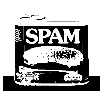
brightness()helper function) is greater than the specifiedthreshold, the pixel should be turned white ([255,255,255]); otherwise, the pixel should be turned black ([0,0,0]).For example, if you do the following:
>>> pixels = load_pixels('spam.png')
>>> bw_spam = bw(pixels, 100)
>>> save_pixels(bw_spam, 'bw_spam.png')
bw_spam.png saved.
you should obtain the following image:
After saving the result of your function, you can double-click on the new PNG file in the
ps7_imagefolder to see the image that was produced. In addition, you should verify that the resulting image is correct by using the procedure explained below.Notes/hints:
-
Your function will need to create a new 2-D list of pixels with the same dimensions as
pixels. You can use theblank_imagefunction that we’ve provided to create a new 2-D list of green pixels that you then modify. -
Your function should return the new 2-D list of pixels that it creates.
-
Important: The 2-D list created by
blank_imagewill be filled with green pixels. If you see unexpected green pixels in your new image (e.g., at the borders of the image), there is a bug in your function that you will need to fix.
Verifying the produced image
The module that we have provided includes a function calledcompare_images()that you can use to test if two images are identical to each other. In addition, we have given you a PNG file for the expected result of each function that you will write.To verify the image produced by your
bw()function, you should do the following after executing the lines above.>>> compare_images('bw_spam.png', 'bw_expected.png') bw_spam.png and bw_expected.png are identical.If the image produced by your
bw()function is identical to the expected result, you will see the message shown above. Otherwise, you will see another message with details about the ways in which the two images differ. -
-
Write a function
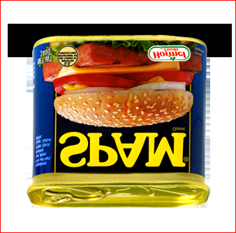
flip_vert(pixels)that takes the 2-D listpixelscontaining pixels for an image, and that creates and returns a new 2-D list of pixels for an image in which the original image is “flipped” vertically. In other words, the top of the original image should now be on the bottom, and the bottom should now be on the top. For example, if you do the following:>>> pixels = load_pixels('spam.png') >>> flipped = flip_vert(pixels) >>> save_pixels(flipped, 'flipv_spam.png') flipv_spam.png saved.
you should obtain the following image:
To verify your image:
>>> compare_images('flipv_spam.png', 'flipv_expected.png')
flipv_spam.png and flipv_expected.png are identical.
Notes/hints:
-
Here again, you should use the
blank_imagefunction to create a new 2-D list of green pixels that you then modify, and you should return the modified 2-D list. -
When computing the appropriate coordinates for a flipped pixel, don’t forget that valid
(r,c)coordinates for an image of heighthand widthware the following:0 ≤ r ≤ h - 1
0 ≤ c ≤ w - 1Given these ranges, where should a pixel from the top row of a given column end up in the flipped image? Where should a pixel from the second row of a given column end up? Where should a pixel from the
rth row of the original image end up?
-
-
Write a function
reduce(pixels)that takes the 2-D listpixelscontaining pixels for an image, and that creates and returns a new 2-D list that represents an image that is half the size of the original image. It should do so by eliminating every other pixel in each row (to reduce the image horizontally) and by eliminating every other row (to reduce the image vertically).There are different approaches that you can take to this problem, and there are two possible results that you can obtain when you reduce a given image. For example, if you do the following:
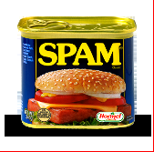
>>> pixels = load_pixels('spam.png')
>>> reduced = reduce(pixels)
>>> save_pixels(reduced, 'reduce_spam.png')
reduce_spam.png saved.
here is one possible result:

Note that the right and bottom borders have been eliminated by the reduction. Here is the other:
In this version, the left and top borders have been eliminated by the reduction. Either result is acceptable.
To help you with testing, we have created an image called
spam_two.pngthat has a two-pixel border: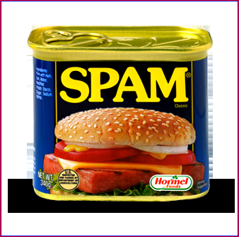
The outermost border is still red, but the inner border is blue.
To verify your function, start by reducing
spam_two.png:>>> pixels = load_pixels('spam_two.png') >>> reduced = reduce(pixels) >>> save_pixels(reduced, 'reduce_spam_two.png') reduce_spam_two.png saved.
You should get one of the following results, either of which is acceptable:

If you get the first of these images, you can verify your image as follows:
>>> compare_images('reduce_spam_two.png', 'reduce_expected.png')
reduce_spam_two.png and reduce_expected.png are identical.
If you get the second of these images, you can verify your image as follows:
>>> compare_images('reduce_spam_two.png', 'reduce2_expected.png')
reduce_spam_two.png and reduce2_expected.png are identical.
Notes/hints:
-
Here again, your function will need to create a new 2-D list of pixels, and you can use the
blank_image()function for that purpose. Use integer division to determine the dimensions of the reduced image. -
One way to solve this problem is to use nested loops to iterate over the rows and columns of the newly created 2-D list–the one that represents the reduced image. You can then perform the necessary computations on your loop variables
randcto determine the cooordinates of the pixel from the original image that you should use for the pixel at position(r, c)in the reduced image. Use concrete cases to determine the appropriate computations.
-
-
Write a function
extract(pixels, rmin, rmax, cmin, cmax)that takes the 2-D listpixelscontaining pixels for an image, and that creates and returns a new 2-D list that represents the portion of the original image that is specified by the other four parameters. The extracted portion of the image should consist of the pixels that fall in the intersection of- the rows of pixels that begin with row
rminand go up to but not including rowrmax - the columns of pixels that begin with column
cminand go up to but not including columncmax.
For example, if you do the following:
>>> pixels = load_pixels('spam.png')
>>> extracted = extract(pixels, 90, 150, 75, 275)
>>> save_pixels(extracted, 'extract_spam.png')
extract_spam.png saved.
you should obtain the following image:

To verify your image:
>>> compare_images('extract_spam.png', 'extract_expected.png')
extract_spam.png and extract_expected.png are identical.
Notes/hints:
-
Here again, your function will need to create and return a new 2-D list of pixels, and you can use the
blank_image()function for that purpose. Compute the dimensions of the new image from the inputs to the function. -
Don’t forget that the
rmaxandcmaxparameters are exclusive, which means that the extracted image should not include pixels from rowrmaxor columncmaxof the original image. This is similar to what happens when you slice a string or list, and it should make it easier to compute the dimensions of the image. -
One way to solve this problem is to use nested loops to iterate over the rows and columns of the newly created 2-D list–the one that represents the extracted image. You can then perform the necessary computations on your loop variables
randcto determine the cooordinates of the pixel from the original image that you should use for the pixel at position(r, c)in the new image. Use concrete cases to determine the appropriate computations.
- the rows of pixels that begin with row
Submitting Your Work
You should use Apollo to submit the following files:
- your
ps7pr0.txtfile containing your response to the reading for Problem 0 - your
ps7pr1.txtfile containing your solution for Problem 1 - your
ps7pr2.pyfile containing your solution for Problem 2 - your
ps7pr3.pyfile containing your solution for Problem 3; if you worked with a partner, make sure that you each submit a copy of your joint work, and that you include comments at the top of the file specifying the name and email of your partner - your
ps7pr4.pyfile containing your solution for Problem 4 - your
ps7pr5.pyfile containing your solution for Problem 5
Note
There is an issue with Apollo that causes print statements with
an end parameter to be deemed a syntax error. The print_grid()
function that we’ve given you includes such a print statement,
so you will probably see an error message when you upload the file
containing that function. You can ignore this message. As long as
your file works correctly when you run it and test it in IDLE, you
should be fine.
Warnings
-
Make sure to use these exact file names, or Apollo will not accept your files. If Apollo reports that a file does not have the correct name, you should rename the file using the name listed in the assignment or on the Apollo upload page.
-
Before submitting your files, make sure that your BU username is visible at the top of the Apollo page. If you don’t see your username, click the Log out button and login again.
-
If you make any last-minute changes to one of your Python files (e.g., adding additional comments), you should run the file in IDLE after you make the changes to ensure that it still runs correctly. Even seemingly minor changes can cause your code to become unrunnable.
-
If you submit an unrunnable file, Apollo will accept your file, but it will print a warning message. If time permits, you are strongly encouraged to fix your file and resubmit. Otherwise, your code will fail most if not all of our tests.
-
If you encounter problems with Apollo, click the Log Out button, close your browser and try again. If possible, you may also want to wait an hour or two before retrying. If you are unable to submit and it is close to the deadline, email your homework before the deadline to
cs111-staff@cs.bu.edu.
Here are the steps:
- Login to Apollo, using the link in the left-hand navigation bar. You will need to use your Kerberos user name and password.
- Check to see that your BU username is at the top of the Apollo page. If it isn’t, click the Log out button and login again.
- Find the appropriate problem set section on the main page and click Upload files.
- For each file that you want to submit, find the matching upload section for the file. Make sure that you use the right section for each file. You may upload any number of files at a time.
- Click the Upload button at the bottom of the page.
- Review the upload results. If Apollo reports any issues, return to the upload page by clicking the link at the top of the results page, and try the upload again, per Apollo’s advice.
- Once all of your files have been successfully uploaded, return to the upload page by clicking the link at the top of the results page. The upload page will show you when you uploaded each file, and it will give you a way to view or download the uploaded file. Click on the link for each file so that you can ensure that you submitted the correct file.
Warning
Apollo will automatically close submissions for a given file when its final deadline has passed. We will not accept any file after Apollo has disabled its upload form, so please check your submission carefully following the instructions in Step 7 above.