Linear Equations
# for QR codes use inline
# %matplotlib inline
# qr_setting = 'url'
#
# for lecture use notebook to manipulate figures
%matplotlib inline
qr_setting = None
#
%config InlineBackend.figure_format='retina'
# import libraries
import numpy as np
import matplotlib as mp
import pandas as pd
import matplotlib.pyplot as plt
import laUtilities as ut
import slideUtilities as sl
import demoUtilities as dm
import pandas as pd
from matplotlib import animation
from importlib import reload
from datetime import datetime
from IPython.display import Image
from IPython.display import display_html
from IPython.display import display
from IPython.display import Math
from IPython.display import Latex
from IPython.display import HTML;
Traditionally, algebra was the art of solving equations and systems of equations. The word algebra comes form the Arabic al-jabr which means restoration (of broken parts). The term was first used in a mathematical sense by Mohammed al-Khowarizmi (c. 780-850) who worked at the House of Wisdom, an academy established by Caliph al Ma’mum in Baghdad. Linear algebra, then, is the art of solving systems of linear equations.
Linear Algebra with Applications , Bretscher
Al-Khowarizmi gave his name to the algorithm. He wrote a book called “ilm al-jabr wa’l-muqābala’ which means “The science of restoring what is missing and equating like with like.”
The central problem of linear algebra is the solution of linear equations.
The yield of one bundle of inferior rice, two bundles of medium grade rice, and three bundles of superior rice is 39 dou of grain. The yield of one bundle of inferior rice, three bundles of medium grade rice, and two bundles of superior rice is 34 dou. The yield of three bundles of inferior rice, two bundles of medium grain rice, and one bundle of superior rice is 26 dou. What is the yield of one bundle of each grade of rice?
Nine Chapters on the Mathematical Art , c 200 BCE, China
# image credit: http://en.wikipedia.org/wiki/The_Nine_Chapters_on_the_Mathematical_Art
display(Image("images/nine-chapters-mathematical-art.jpg",width=300))
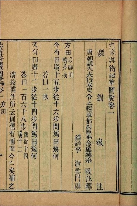
HTML(u'<a href="http://commons.wikimedia.org/wiki/File:%E4%B9%9D%E7%AB%A0%E7%AE%97%E8%A1%93%E7%B4%B0%E8%8D%89%E5%9C%96%E8%AA%AA.jpg#/media/File:%E4%B9%9D%E7%AB%A0%E7%AE%97%E8%A1%93%E7%B4%B0%E8%8D%89%E5%9C%96%E8%AA%AA.jpg">九章算術細草圖說</a> by 中國書店海王邨公司 - <a rel="nofollow" class="external free" href="http://pmgs.kongfz.com/detail/1_158470/">http://pmgs.kongfz.com/detail/1_158470/</a>. Licensed under Public Domain via <a href="//commons.wikimedia.org/wiki/">Wikimedia Commons</a>.')
Let’s denote the unknown quantities as \(x_1\), \(x_2\), and \(x_3\). These are the yields of one bundle of inferior, medium grade, and superior rice, respectively. We can then write the problem as:
The problem then is to determine the values of \(x_1, x_2,\) and \(x_3\).
These are linear equations. No term has power other than 1.
For example, there are no terms involving \(x_1^2\), or \(x_1x_2\), or \(\sqrt{x_3}\).
Basic Definitions
A linear equation in the variables \(x_1, \dots, x_n\) is an equation that can be written in the form
where \(b\) and the coefficients \(a_1, \dots, a_n\) are real or complex numbers that are usually known in advance.
A system of linear equations (or linear system ) is a collection of one or more linear equations involving the same variables - say \(x_1, \dots, x_n\).
A solution of the system is a list of numbers \((s_1, s_2, \dots, s_n)\) that makes each equation a true statement when the values \(s_1, s_2, \dots, s_n\) are substituted for \(x_1, x_2, \dots, x_n,\) respectively.
The set of all possible solutions is called the solution set of the linear system.
Two linear systems are called equivalent if they have the same solution set.
A system of linear equations has
no solution, or
exactly one solution, or
infinitely many solutions.
A system of linear equations is said to be consistent if it has either one solution or infinitely many solutions.
A system of linear equations is said to be inconsistent if it has no solution.
The Geometry of Linear Equations
Any list of numbers \((s_1, s_2, \dots, s_n)\) can be thought of as a point in \(n\)-dimensional space, called a vector space.
We call that vector space \(\mathbb{R}^n\).
So if we are considering linear equations with \(n\) unknowns, the solutions are points in \(\mathbb{R}^n\).
Now, any linear equation defines a point set with dimension one less than the space. For example:
if we are in 2-space (2 unknowns), a linear equation defines a line.
if we are in 3-space (3 unknowns), a linear equation defines a plane.
in higher dimensions, we refer to all such sets as hyperplanes.
Question: why does a linear equation define a point-set of dimension one less than the space?
Some Examples in \(\mathbb{R}^2\)
How many solutions does the linear system have in each case?
fig = ut.two_d_figure('Figure 1.2d.1', size = (6,6))
fig.centerAxes()
fig.plotLinEqn( 1, -2, -1, color = 'r')
fig.plotLinEqn(-1,  3,  3, color = 'b')
plt.legend(loc='best', fontsize = 14);
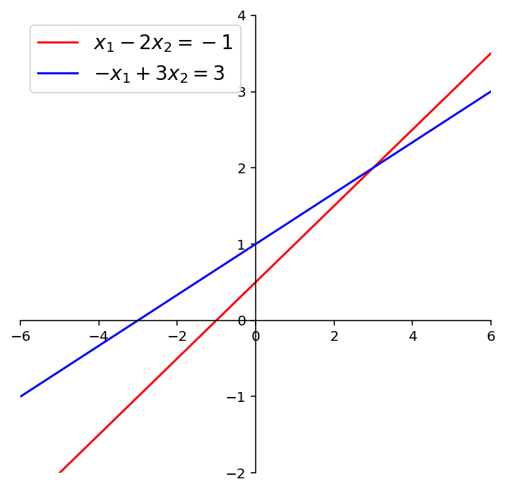
This system of two equations has exactly one solution.
fig = ut.two_d_figure('Figure 1.2d.2', size = (6,6))
fig.centerAxes()
fig.plotLinEqn( 1, -2, -1, color = 'r')
fig.plotLinEqn(-1,  2,  3, color = 'b')
plt.legend(loc='best', fontsize = 14);
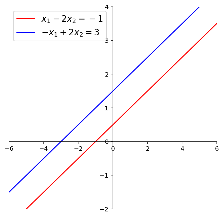
This system of two equations has no solutions.
fig = ut.two_d_figure('Figure 1.2d.3', size = (6,6))
fig.centerAxes()
fig.plotLinEqn( 1, -2, -1, color = 'r')
fig.plotLinEqn(-1,  2,  1, format = '--', color = 'b')
plt.legend(loc='best', fontsize = 14);
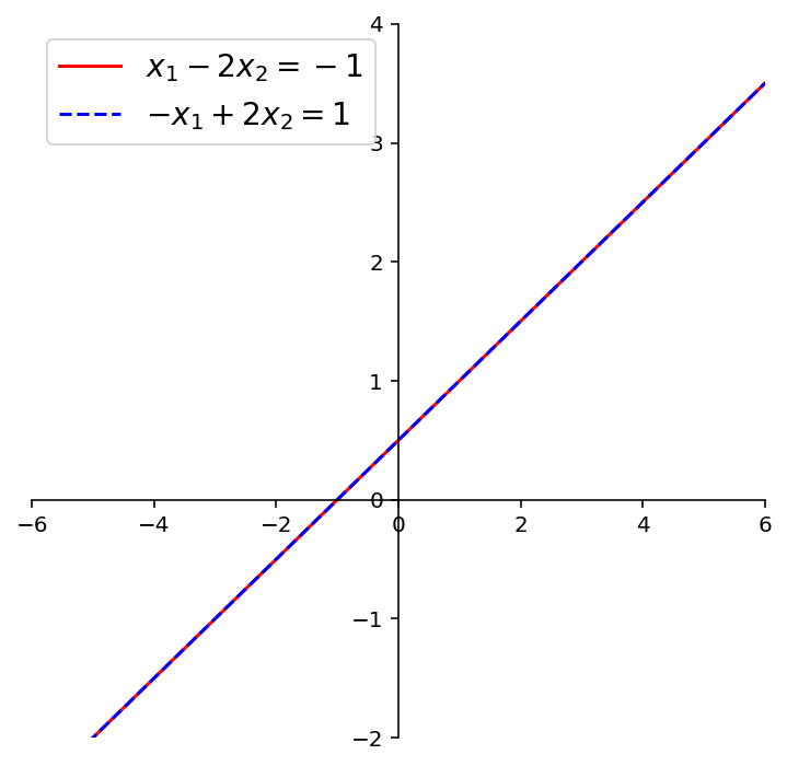
This system of equations has infinitely many solutions.
Some Examples in \(\mathbb{R}^3\)
How many solutions are there in each of these cases?
fig = ut.three_d_figure((1, 1), fig_desc = 'Example 1: One Solution',
                        xmin = -5, xmax = 5, ymin = -5, ymax = 5, zmin = -5, zmax = 5,
                        figsize = (6,6), qr = qr_setting, displayAxes = False)
eq1 = [1, 0, 0,  1]
eq2 = [0, 1, 0, -2]
eq3 = [0, 0, 1,  0]
fig.plotLinEqn(eq1, 'Brown')
fig.plotLinEqn(eq2, 'Green')
fig.plotLinEqn(eq3, 'Blue')
fig.plotIntersection(eq1, eq2, color='Blue', line_type='--')
fig.plotIntersection(eq2, eq3, color='Blue', line_type='--')
fig.plotIntersection(eq1, eq3, color='Blue', line_type='--')
fig.set_title('Example 1')
fig.save()
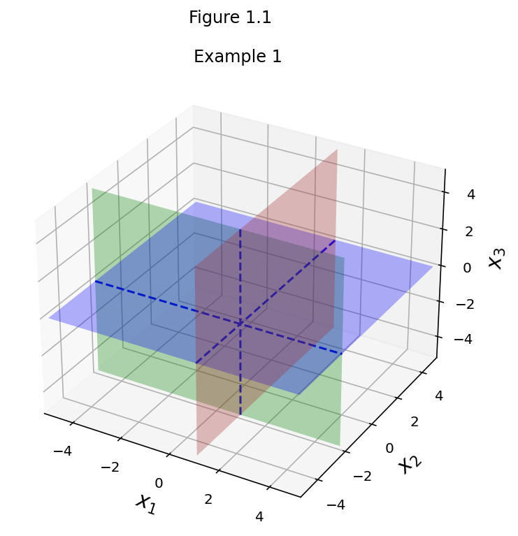
fig = ut.three_d_figure((1, 2), fig_desc = 'Example 2: No Solutions',
                        xmin = -5, xmax = 5, ymin = -5, ymax = 5, zmin = -5, zmax = 5,
                        figsize = (6,6), qr = qr_setting, displayAxes = False)
# equation of a line from its normal a is a'x = a'a
# three normals 120 degrees spread around the y axis
eq1 = [np.sqrt(3/4),  0, 1/2,  1]
eq2 = [-np.sqrt(3/4), 0, 1/2,  1]
eq3 = [0,                 0, -1,       2]
fig.plotLinEqn(eq1, 'Brown')
fig.plotLinEqn(eq2, 'Green')
fig.plotLinEqn(eq3, 'Blue')
fig.plotIntersection(eq1, eq2, color='Blue', line_type='--')
fig.plotIntersection(eq2, eq3, color='Blue', line_type='--')
fig.plotIntersection(eq1, eq3, color='Blue', line_type='--')
fig.set_title('Example 2')
fig.save()
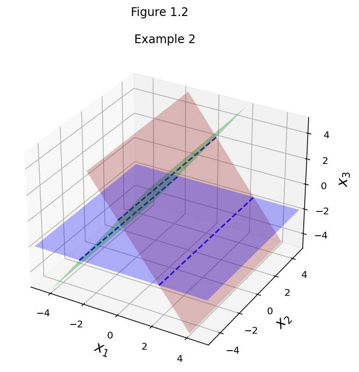
fig = ut.three_d_figure((1, 3), fig_desc = 'Example 3: Infinite Number of Solutions',
                        xmin = -5, xmax = 5, ymin = -5, ymax = 5, zmin = -5, zmax = 5,
                        figsize = (6,6), qr = qr_setting, displayAxes = False)
# equation of a line from its normal a is a'x = a'a
# three normals 120 degrees spread around the y axis
eq1 = [np.sqrt(3/4),  0, 1/2,  0]
eq2 = [-np.sqrt(3/4), 0, 1/2,  0]
eq3 = [0,             0,  -1,  0]
fig.plotLinEqn(eq1, 'Brown')
fig.plotLinEqn(eq2, 'Green')
fig.plotLinEqn(eq3, 'Blue')
fig.plotIntersection(eq1, eq2, color='Blue', line_type='--')
fig.plotIntersection(eq2, eq3, color='Blue', line_type='--')
fig.plotIntersection(eq1, eq3, color='Blue', line_type='--')
fig.set_title('Example 3')
fig.save()
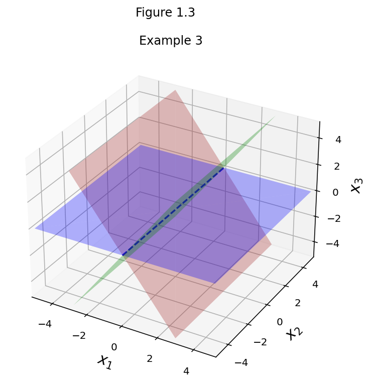
fig = ut.three_d_figure((1, 4), fig_desc = 'Example 4: No Solutions',
                        xmin = -5, xmax = 5, ymin = -5, ymax = 5, zmin = -5, zmax = 5,
                        figsize = (6,6), qr = qr_setting, displayAxes = False)
# equation of a line from its normal a is a'x = a'a
# three normals 120 degrees spread around the y axis
eq1 = [np.sqrt(3/4),  0, 1/2,  0]
eq2 = [np.sqrt(3/4),  0, 1/2,  2]
eq3 = [np.sqrt(3/4),  0, 1/2,  -2]
fig.plotLinEqn(eq1, 'Brown')
fig.plotLinEqn(eq2, 'Green')
fig.plotLinEqn(eq3, 'Blue')
# fig.plotIntersection(eq1, eq2, color='Blue', line_type='--')
# fig.plotIntersection(eq2, eq3, color='Blue', line_type='--')
# fig.plotIntersection(eq1, eq3, color='Blue', line_type='--')
fig.set_title('Example 4')
fig.save()
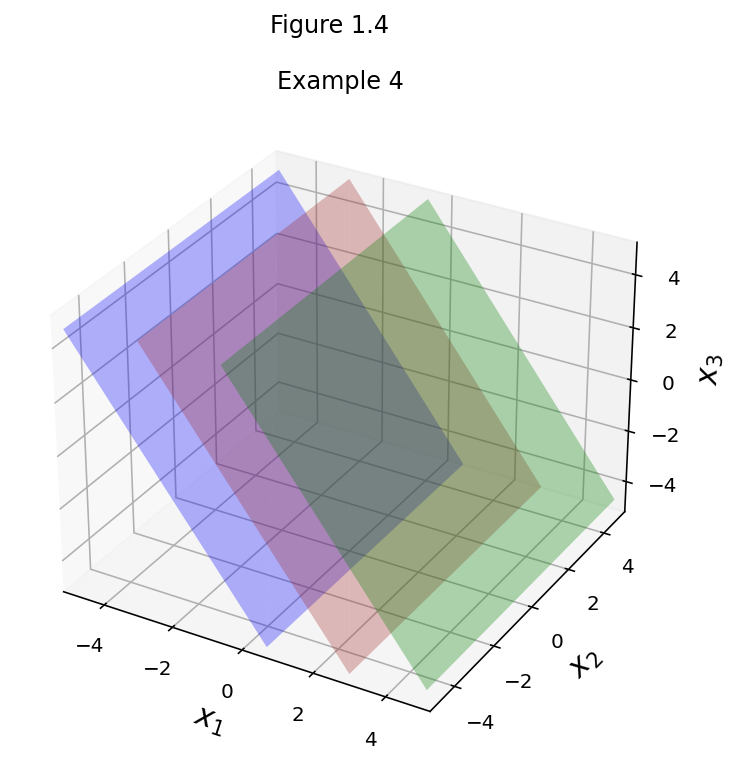
fig = ut.three_d_figure((1, 5), fig_desc = 'Example 5: No Solutions',
                        xmin = -5, xmax = 5, ymin = -5, ymax = 5, zmin = -5, zmax = 5,
                        figsize = (6,6), qr = qr_setting, displayAxes = False)
# equation of a line from its normal a is a'x = a'a
# three normals 120 degrees spread around the y axis
eq1 = [np.sqrt(4/3),  0, -2,  0]
eq2 = [np.sqrt(3/4),  0, 1/2,  2]
eq3 = [np.sqrt(3/4),  0, 1/2,  -2]
fig.plotLinEqn(eq1, 'Brown')
fig.plotLinEqn(eq2, 'Green')
fig.plotLinEqn(eq3, 'Blue')
fig.plotIntersection(eq1, eq2, color='Blue', line_type='--')
# fig.plotIntersection(eq2, eq3, color='Blue', line_type='--')
fig.plotIntersection(eq1, eq3, color='Blue', line_type='--')
fig.set_title('Example 5')
fig.save()
The Matrices of a System
The essential information of a linear system can be recorded compactly in a rectangular array called a matrix. For the following system of equations,
the matrix
is called the coefficient matrix of the system.
An augmented matrix of a system consists of the coefficient matrix with an added column containing the constants from the right sides of the equations.
For the same system of equations,
the matrix
is called the augmented matrix of the system.
A matrix with \(m\) rows and \(n\) columns is referred to as ‘’an \(m \times n\) matrix’’ and is an element of the set \(\mathbb{R}^{m\times n}.\)
(Note that we always list the number of rows first, then the number of columns.)
Question Time! Q1.1
Solving Linear Systems
To solve a linear system, we transform it into a new system which is equivalent to the old system, meaning it has the same solution set.
However, in the new system the solution is explicit.
We can make these transformations because of three facts.
Fact Number 1: Given a set of linear equations, we can add one equation to another without changing the solution set.
By definition, any solution of the old system makes each old equation true; therefore any solution of the old system makes each new equation true.
Example:
This has the same solution set as:
Fact Number 2: Another, more obvious fact is that we can multiply any equation by a constant without changing its meaning (and therefore the solution set).
Example:
has the same solution set as:
Fact Number 3: And an even more obvious fact is that we can change the order of the equations without changing anything.
Together, these three rules form a set of tools we can use to solve linear systems. Here is an example.
Step 1: Elimination
The process we’ll describe consists of two steps: Elimination and Backsubstitution.
The goal of elimination is to eliminate terms to create a triangular matrix (or system). The basic operation we will repeatedly apply is to add a multiple of one equation (row) to another. We’ll do this with the equations and the matrix side-by-side.
Here is the original system:
The first stage of the process is called elimination. To begin: we add -6 times the first equation to the third equation:
This gives us a new system.
Note that this is not the same system of equations, but it is equivalent – it has the same solution set.
Next, we multiply the second equation by \(1/2\) to get its leading coefficient to be 1:
Next, we multiply the second equation by \(-17\) and add it to the third equation:
And next we can divide the third equation by \(71\) to get its leading coefficient equal to 1:
We have now put the system and matrix into triangular form. In a triangular matrix, all values below the diagonal are zero.
Step 2: Backsubstitution
At this point, the process shifts to backsubstitution. We now have the value for one variable, and we will substitute it into other equations to simplify them and get values for the other variables.
Although we think of its as a somewhat different stage, in reality it still comes down to applying the three rules.
First, we substitute the value of \(x_3\) into the equations above it. This is actually multiplying equation 3 by the proper value and adding it to equations above it.
Next, we do the same thing with equation 2, substituting it into equation 1 above it:
Now we can read off the solution: it is \(x_1 = 1\), \(x_2 = -2\), \(x_3 = 0\). Notice the particular form of the resulting matrix: ones on the diagonal, zeros above and below each 1.
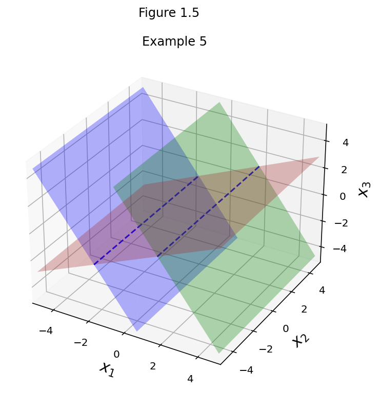
Let’s get a sense of this process geometrically.
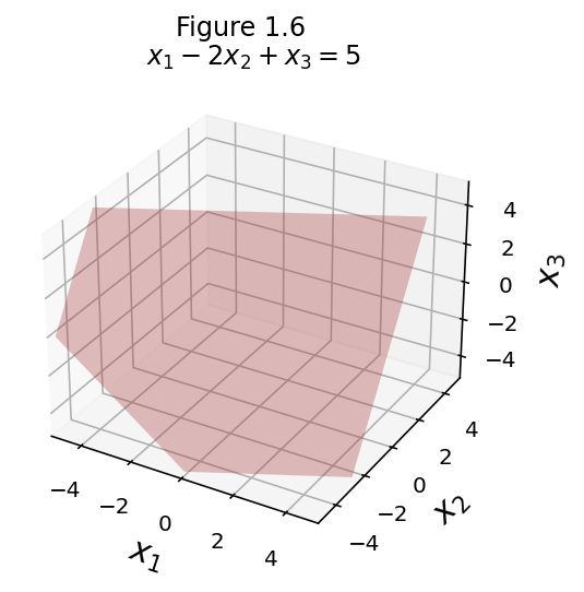
Here are the three starting equations:
eq1 = [1, -2, 1, 5]
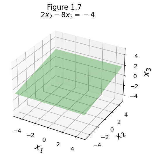
eq2 = [0, 2, -8, -4]
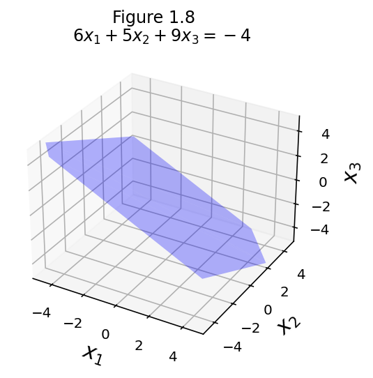
eq3 = [6, 5, 9, -4]
fig = ut.three_d_figure((1, 6), fig_desc = format(ut.formatEqn(eq1[0:3], eq1[3])),
xmin = -5, xmax = 5, ymin = -5, ymax = 5, zmin = -5, zmax = 5, qr = qr_setting)
fig.plotLinEqn(eq1, 'Brown')
fig.set_title('${}$'.format(ut.formatEqn(eq1[0:3], eq1[3])))
fig.save()
fig = ut.three_d_figure((1, 7), format(ut.formatEqn(eq2[0:3], eq2[3])),
xmin = -5, xmax = 5, ymin = -5, ymax = 5, zmin = -5, zmax = 5, qr = qr_setting)
fig.plotLinEqn(eq2, 'Green')
fig.set_title('${}$'.format(ut.formatEqn(eq2[0:3], eq2[3])))
fig.save()
fig = ut.three_d_figure((1, 8), fig_desc = format(ut.formatEqn(eq3[0:3], eq3[3])),
xmin = -5, xmax = 5, ymin = -5, ymax = 5, zmin = -5, zmax = 5, qr = qr_setting)
fig.plotLinEqn(eq3, 'Blue')
fig.set_title('${}$'.format(ut.formatEqn(eq3[0:3], eq3[3])))
fig.save()
Now let’s compare the starting point and the finishing point:
fig = ut.three_d_figure((1, 9), fig_desc = 'All Three Equations',
                        xmin = -5, xmax = 5, ymin = -5, ymax = 5, zmin = -5, zmax = 5, qr = qr_setting)
eq1 = [1, -2,  1,  5]
eq2 = [0,  2, -8, -4]
eq3 = [6,  5,  9, -4]
fig.plotLinEqn(eq1, 'Brown')
fig.plotLinEqn(eq2, 'Green')
fig.plotLinEqn(eq3, 'Blue')
fig.plotIntersection(eq1, eq2, color='Blue', line_type='--')
fig.plotIntersection(eq2, eq3, color='Blue', line_type='--')
fig.plotIntersection(eq1, eq3, color='Blue', line_type='--')
fig.plotPoint(1, -2, 0)
fig.set_title('All Three Equations')
fig.save()

fig = ut.three_d_figure((1, 10), fig_desc = 'The Equivalent System',
                        xmin = -5, xmax = 5, ymin = -5, ymax = 5, zmin = -5, zmax = 5, qr = qr_setting)
eq1 = [1, 0, 0,  1]
eq2 = [0, 1, 0, -2]
eq3 = [0, 0, 1,  0]
fig.plotLinEqn(eq1, 'Brown')
fig.plotLinEqn(eq2, 'Green')
fig.plotLinEqn(eq3, 'Blue')
fig.plotIntersection(eq1, eq2, color='Blue', line_type='--')
fig.plotIntersection(eq2, eq3, color='Blue', line_type='--')
fig.plotIntersection(eq1, eq3, color='Blue', line_type='--')
fig.plotPoint(1, -2, 0)
fig.set_title('The Equivalent System')
fig.save()
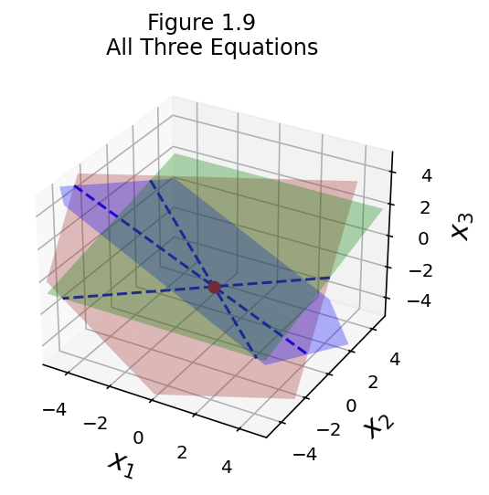
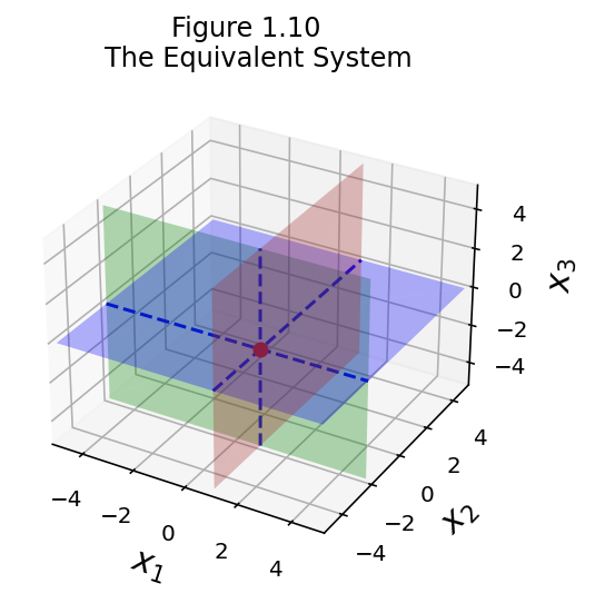
Notice how all the planes have shifted, but they still intersect in the same point. This is the geometric interpretation of equivalent systems.
Verifying the Solution
It’s important that, once you have solved a system, you verify the solution
i.e., go back and confirm that what you have computed, in fact meets the original requirements.
So, in our case here is the original system and its solution:
We can verify by substitution:
The solution \((1, -2, 0)\) makes each equation true. Confirmed!
Row Equivalence
OK, let’s step back and formalize what we have done.
Elementary Row Operations are the following:
(Replacement) Replace one row by the sum of itself and a multiple of another row.
(Interchange) Interchange two rows.
(Scaling) Multiply all entries in a row by a nonzero constant.
Two matrices are called row equivalent if there is a sequence of elementary row operations that transforms one matrix into the other.
If the augmented matrices of two linear systems are row equivalent, then the two systems have the same solution set.
Fundamental Questions
When presented with a linear system, we always need to ask two fundamental questions:
Is the system consistent; that is, does at least one solution exist?
If a solution exists, is there only one; that is, is the solution unique?
These really are fundamental; we will see that the answers to these questions have far-reaching implications.
Recognizing an Inconsistent System
Consider the following system:
whose augmented matrix is:
Let’s apply our row reduction procedure to this matrix.
First, we’ll interchange rows 1 and 2:
Next, we’ll eliminate the \(4x_1\) term in the third equation by adding \(-2\) times row 1 to row 3:
Next, we use the \(x_2\) term in the second equation to eliminate the \(-2x_2\) term from the third equation (that is, add 2 times row 2 to row 3).
This matrix is now in triangular form.
What does it mean? In particular, what does the last row say?
The last row stands for the equation:
Clearly, this equation has no solution. Now, we know that row reductions never change the solution set of a system. So, the original set of equations also has no solution. It is inconsistent.
We can conclude that an inconsistent system will lead, by row reductions, to a system containing the equation \(0 = k\) for some nonzero \(k\).
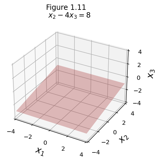
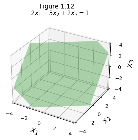
Geometric Interpretation of Inconsistency
Here are our original equations, as hyperplanes:
eq1 = [0, 1, -4, 8]
eq2 = [2, -3, 2, 1]
eq3 = [5, -8, 7, -20]
fig = ut.three_d_figure((1, 11), fig_desc = format(ut.formatEqn(eq1[0:3], eq1[3])),
xmin = -4, xmax = 4, ymin = -4, ymax = 4, zmin = -4, zmax = 4, qr = qr_setting)
fig.plotLinEqn(eq1, 'Brown')
fig.set_title('${}$'.format(ut.formatEqn(eq1[0:3], eq1[3])))
fig.save()
fig = ut.three_d_figure((1, 12), fig_desc = format(ut.formatEqn(eq2[0:3], eq2[3])),
xmin = -4, xmax = 4, ymin = -4, ymax = 4, zmin = -4, zmax = 4, qr = qr_setting)
fig.plotLinEqn(eq2, 'Green')
fig.set_title('${}$'.format(ut.formatEqn(eq2[0:3], eq2[3])))
fig.save()
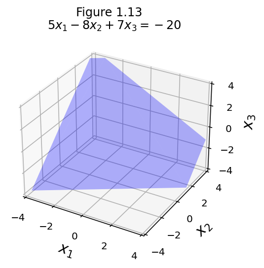
fig = ut.three_d_figure((1, 13), fig_desc = format(ut.formatEqn(eq3[0:3], eq3[3])),
xmin = -4, xmax = 4, ymin = -4, ymax = 4, zmin = -4, zmax = 4, qr = qr_setting)
fig.plotLinEqn(eq3, 'Blue')
fig.set_title('${}$'.format(ut.formatEqn(eq3[0:3], eq3[3])))
fig.save()
Here is a view of all three hyperplanes.
fig = ut.three_d_figure((1, 14), fig_desc = 'All Three Equations',
                        xmin = -5, xmax = 5, ymin = -5, ymax = 5, zmin = -5, zmax = 5, qr = qr_setting)
fig.plotLinEqn(eq1, 'Brown')
fig.plotLinEqn(eq2, 'Green')
fig.plotLinEqn(eq3, 'Blue')
fig.plotIntersection(eq1, eq2, color='Blue')
fig.plotIntersection(eq1, eq3, color='Blue')
fig.set_title('All Three Equations')
fig.ax.view_init(azim=45)
fig.save()
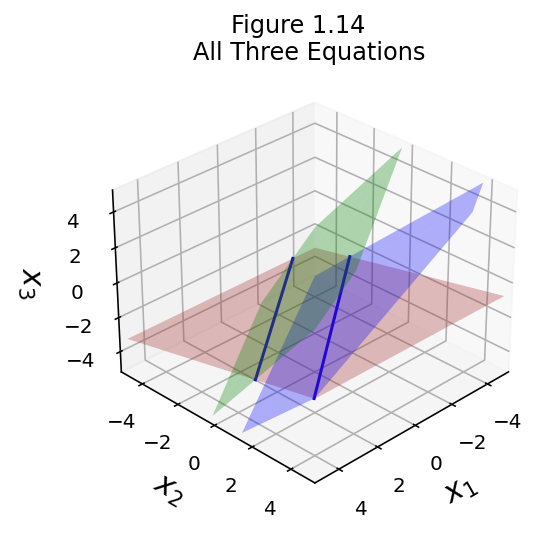
The figure illustrates that the two intersection lines are parallel. So there is no point that lies in all the hyperplanes. That is the geometric interpretation of inconsistency.
Summary
Our entry into linear algebra has been through the solution of systems of linear equations.
We used a tabular representation called a matrix to represent the linear system
The solution method uses matrix row reductions: exchanging rows, scaling rows, or adding rows.
The solution method has two stages: elimination and backsubstitution.
We observed some basic properties of linear systems:
They can be consistent or inconsistent.
If consistent, they can have a single solution or an infinite number of solutions.
We thought geometrically about linear systems and their solutions:
A linear equation defines a hyperplane
In a consistent system, all hyperplanes intersect in one or more points
In an inconsistent system, all hyperplanes do not intersect in any single point
The solution method we used creates hyperplanes that intersect in the same point set as the original hyperplanes