# for QR codes use inline
%matplotlib inline
qr_setting = 'url'
#
# for lecture use notebook
# %matplotlib notebook
# qr_setting = None
#
%config InlineBackend.figure_format='retina'
# import libraries
import numpy as np
import matplotlib as mp
import pandas as pd
import matplotlib.pyplot as plt
import laUtilities as ut
import slideUtilities as sl
import demoUtilities as dm
import pandas as pd
from importlib import reload
from datetime import datetime
from IPython.display import Image
from IPython.display import display_html
from IPython.display import display
from IPython.display import Math
from IPython.display import Latex
from IPython.display import HTML;
The Matrix of a Linear Transformation
# image credit: https://imgflip.com/memetemplate/The-Most-Interesting-Man-In-The-World
display(Image("images/Dos-Equis-Linear-Transform.jpg", width=350))

In the last lecture we introduced the idea of a linear transformation:
# image credit: Lay, 4th edition
display(Image("images/L7 F4.jpg", width=650))

We have seen that every matrix multiplication is a linear transformation from vectors to vectors.
But, are there any other possible linear transformations from vectors to vectors?
No.
In other words, the reverse statement is also true:
every linear transformation from vectors to vectors is a matrix multiplication.
We’ll now prove this fact. We’ll do it constructively, meaning we’ll actually show how to find the matrix corresponding to any given linear transformation \(T\).
Theorem. Let \(T: \mathbb{R}^n \rightarrow \mathbb{R}^m\) be a linear transformation. Then there is (always) a unique matrix \(A\) such that:
In fact, \(A\) is the \(m \times n\) matrix whose \(j\)th column is the vector \(T({\bf e_j})\), where \({\bf e_j}\) is the \(j\)th column of the identity matrix in \(\mathbb{R}^n\):
\(A\) is called the standard matrix of \(T\).
Proof. Write
Because \(T\) is linear, we have:
So … we see that the ideas of matrix multiplication and linear transformation are essentially equivalent.
However, term linear transformation focuses on a property of the mapping, while the term matrix multiplication focuses on how such a mapping is implemented.
This proof shows us an important idea:
To find the standard matrix of a linear tranformation, ask what the transformation does to the columns of \(I\).
Now, in \(\mathbb{R}^2\), \(I = \left[\begin{array}{cc}1&0\\0&1\end{array}\right]\). So:
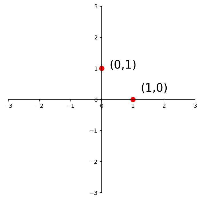
So to find the matrix of any given linear transformation of vectors in \(\mathbb{R}^2\), we only have to know what that transformation does to these two points:
ax = dm.plotSetup(-3,3,-3,3,size=(6,6))
ax.plot([0],[1],'ro',markersize=8)
ax.text(0.25,1,'(0,1)',size=20)
ax.plot([1],[0],'ro',markersize=8)
ax.text(1.25,0.25,'(1,0)',size=20);

This is a hugely powerful tool.
Let’s say we start from some given linear transformation; we can use this idea to find the matrix that implements that linear transformation.
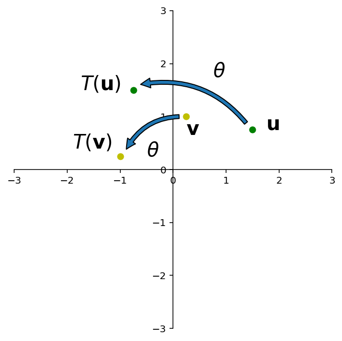
For example, let’s consider rotation about the origin as a kind of transformation.
u = np.array([1.5, 0.75])
v = np.array([0.25, 1])
diamond = np.array([[0,0], u,  u+v, v]).T
ax = dm.plotSetup()
plt.plot(u[0], u[1], 'go')
plt.plot(v[0], v[1], 'yo')
ax.text(u[0]+.25,u[1],r'$\bf{u}$',size=20)
ax.text(v[0],v[1]-.35,r'$\bf{v}$',size=20)
rotation = np.array([[0, -1],[1, 0]])
up = rotation @ u
vp = rotation @ v
plt.plot(up[0], up[1], 'go')
plt.plot(vp[0], vp[1], 'yo')
ax.text(up[0]-1,up[1],r'$T(\mathbf{u})$',size=20)
ax.text(vp[0]-.9,vp[1]+.15,r'$T(\mathbf{v})$',size=20)
ax.text(0.75, 1.75, r'$\theta$', size = 20)
ax.text(-.5, 0.25, r'$\theta$', size = 20)
ax.annotate("",
            xy=((up)[0]+.1, (up)[1]+.1), xycoords='data',
            xytext=((u)[0]-.1, (u)[1]+.1), textcoords='data',
            size=20, va="center", ha="center",
            arrowprops=dict(arrowstyle="simple",
                            connectionstyle="arc3,rad=0.3"),
            )
ax.annotate("",
            xy=((vp)[0]+.1, (vp)[1]+.1), xycoords='data',
            xytext=((v)[0]-.1, (v)[1]), textcoords='data',
            size=20, va="center", ha="center",
            arrowprops=dict(arrowstyle="simple",
                            connectionstyle="arc3,rad=0.3"),
            );
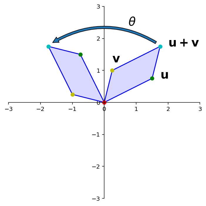
First things first: Is rotation a linear transformation?
Recall that a for a transformation to be linear, it must be true that \(T(\mathbf{u} + \mathbf{v}) = T(\mathbf{u}) + T(\mathbf{v}).\)
I’m going to show you a “geometric proof.”
This figure shows that “the rotation of \(\mathbf{u+v}\) is the sum of the rotation of \(\mathbf{u}\) and the rotation of \(\mathbf{v}\)”.
u = np.array([1.5, 0.75])
v = np.array([0.25, 1])
diamond = np.array([[0,0], u,  u+v, v]).T
ax = dm.plotSetup()
dm.plotSquare(diamond)
ax.text(u[0]+.25,u[1],r'$\bf{u}$',size=20)
ax.text(v[0],v[1]+.25,r'$\bf{v}$',size=20)
ax.text(u[0]+v[0]+.25,u[1]+v[1],r'$\bf{u + v}$',size=20)
rotation = np.array([[0, -1],[1, 0]])
up = rotation @ u
vp = rotation @ v
diamond = np.array([[0,0], up,  up+vp, vp]).T
dm.plotSquare(diamond)
ax.text(0.75, 2.4, r'$\theta$', size = 20)
ax.annotate("",
            xy=((up+vp)[0]+.1, (up+vp)[1]+.1), xycoords='data',
            xytext=((u+v)[0]-.1, (u+v)[1]+.1), textcoords='data',
            size=20, va="center", ha="center",
            arrowprops=dict(arrowstyle="simple",
                            connectionstyle="arc3,rad=0.3"),
            );
OK, so rotation is a linear transformation.
Let’s see how to compute the linear transformation that is a rotation.
Specifically: Let \(T: \mathbb{R}^2 \rightarrow \mathbb{R}^2\) be the transformation that rotates each point in \(\mathbb{R}^2\) about the origin through an angle \(\theta\), with counterclockwise rotation for a positive angle.
Let’s find the standard matrix \(A\) of this transformation.
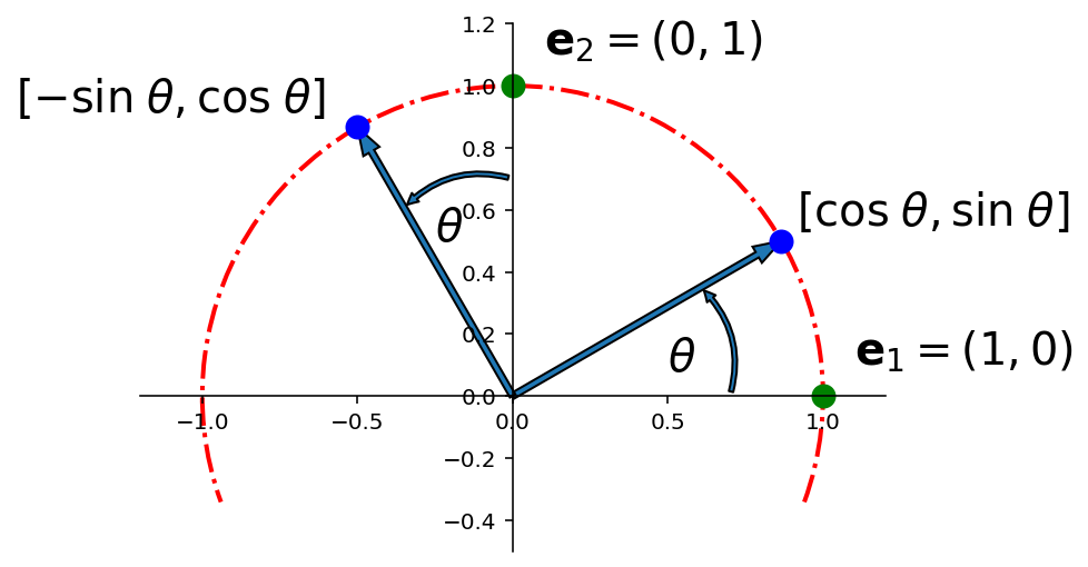
Solution. The columns of \(I\) are \({\bf e_1} = \left[\begin{array}{r}1\\0\end{array}\right]\) and \({\bf e_2} = \left[\begin{array}{r}0\\1\end{array}\right].\)
Referring to the diagram below, we can see that \(\left[\begin{array}{r}1\\0\end{array}\right]\) rotates into \(\left[\begin{array}{r}\cos\theta\\\sin\theta\end{array}\right],\) and \(\left[\begin{array}{r}0\\1\end{array}\right]\) rotates into \(\left[\begin{array}{r}-\sin\theta\\\cos\theta\end{array}\right].\)
import matplotlib.patches as patches
ax = dm.plotSetup(-1.2, 1.2, -0.5, 1.2)
# red circle portion
arc = patches.Arc([0., 0.], 2., 2., 0., 340., 200.,
                 linewidth = 2, color = 'r',
                 linestyle = '-.')
ax.add_patch(arc)
#
# labels
ax.text(1.1, 0.1, r'$\mathbf{e}_1 = (1, 0)$', size = 20)
ax.text(0.1, 1.1, r'$\mathbf{e}_2 = (0, 1)$', size = 20)
#
# angle of rotation and rotated points
theta = np.pi / 6
e1t = [np.cos(theta), np.sin(theta)]
e2t = [-np.sin(theta), np.cos(theta)]
#
# theta labels
ax.text(0.5, 0.08, r'$\theta$', size = 20)
ax.text(-0.25, 0.5, r'$\theta$', size = 20)
#
# arrows from origin
ax.arrow(0, 0, e1t[0], e1t[1],
        length_includes_head = True,
        width = .02)
ax.arrow(0, 0, e2t[0], e2t[1],
        length_includes_head = True,
        width = .02)
#
# new point labels
ax.text(e1t[0]+.05, e1t[1]+.05, r'$[\cos\; \theta, \sin \;\theta]$', size = 20)
ax.text(e2t[0]-1.1, e2t[1]+.05, r'$[-\sin\; \theta, \cos \;\theta]$', size = 20)
#
# curved arrows showing rotation
ax.annotate("",
            xytext=(0.7, 0), xycoords='data',
            xy=(0.7*e1t[0], 0.7*e1t[1]), textcoords='data',
            size=10, va="center", ha="center",
            arrowprops=dict(arrowstyle="simple",
                            connectionstyle="arc3,rad=0.3"),
            )
ax.annotate("",
            xytext=(0, 0.7), xycoords='data',
            xy=(0.7*e2t[0], 0.7*e2t[1]), textcoords='data',
            size=10, va="center", ha="center",
            arrowprops=dict(arrowstyle="simple",
                            connectionstyle="arc3,rad=0.3"),
            )
#
# new points
plt.plot([e1t[0], e2t[0]], [e1t[1], e2t[1]], 'bo', markersize = 10)
plt.plot([0, 1], [1, 0], 'go', markersize = 10);
So by the Theorem above,
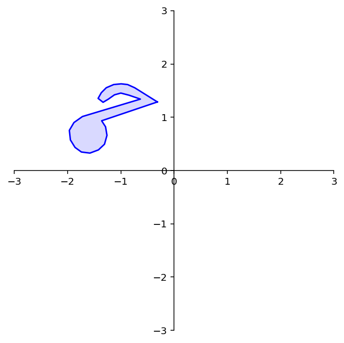
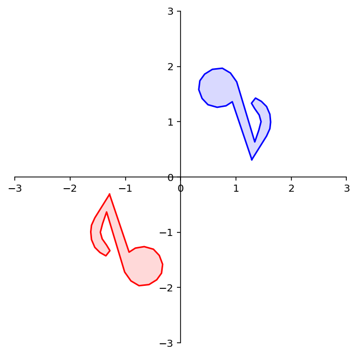
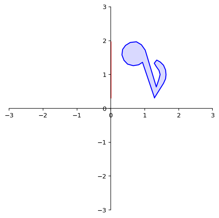
To demonstrate the use of a rotation matrix, let’s rotate the following shape:
dm.plotSetup()
note = dm.mnote()
dm.plotShape(note)
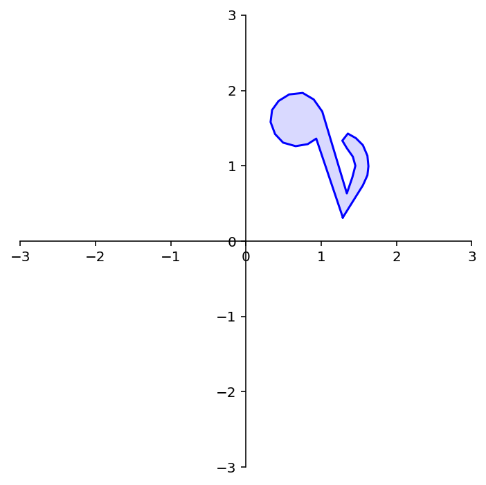
The variable note is a array of 26 vectors in \(\mathbb{R}^2\) that define its shape.
In other words, it is a 2 \(\times\) 26 matrix.
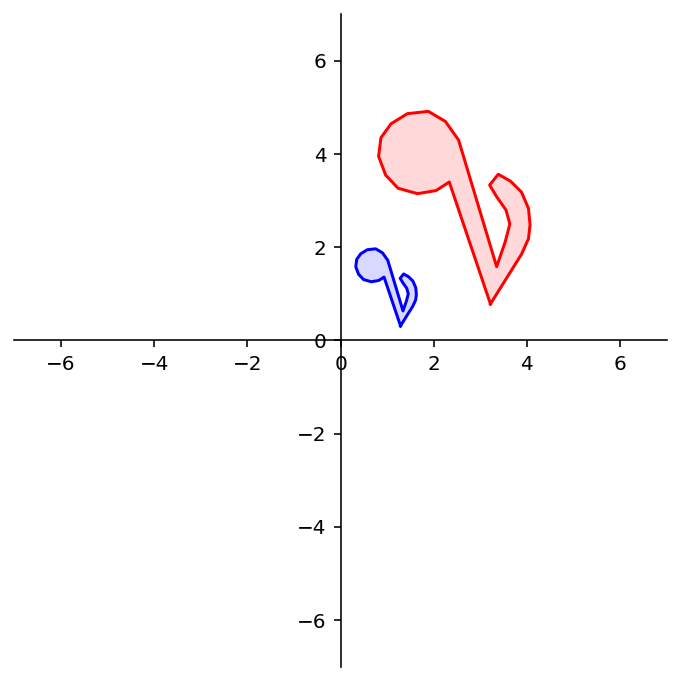
To rotate note we need to multiply each column of note by the rotation matrix \(A\).
In Python matrix multiplication is performed using the @ operator.
That is, if A and B are matrices,
A @ B
will multiply A by every column of B, and the resulting vectors will be formed
into a matrix.
dm.plotSetup()
angle = 90
theta = (angle/180) * np.pi
A = np.array(
    [[np.cos(theta), -np.sin(theta)],
     [np.sin(theta), np.cos(theta)]])
rnote = A @ note
dm.plotShape(rnote)
Geometric Linear Transformations of \(\mathbb{R}^2\)
Let’s use our understanding of how to constuct linear transformations to look at some specific linear transformations of \(\mathbb{R}^2\) to \(\mathbb{R}^2\).
First, let’s recall the linear transformation
With \(r > 1\), this is a dilation. It moves every vector further from the origin.
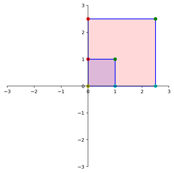
Let’s say the dilation is by a factor of 2.5.
To construct the matrix \(A\) that implements this transformation, we ask: where do \({\bf e_1}\) and \({\bf e_2}\) go?
ax = dm.plotSetup()
ax.plot([0],[1],'ro',markersize=8)
ax.text(0.25,1,'(0,1)',size=20)
ax.plot([1],[0],'ro',markersize=8)
ax.text(1.25,0.25,'(1,0)',size=20);
Under the action of \(A\), \(\mathbf{e_1}\) goes to \(\left[\begin{array}{c}2.5\\0\end{array}\right]\) and \(\mathbf{e_2}\) goes to \(\left[\begin{array}{c}0\\2.5\end{array}\right]\).
So the matrix \(A\) must be \(\left[\begin{array}{cc}2.5&0\\0&2.5\end{array}\right]\).
Let’s test this out:
square = np.array(
    [[0,1,1,0],
     [1,1,0,0]])
A = np.array(
    [[2.5, 0],
     [0, 2.5]])
print('A = \n',A)
dm.plotSetup()
dm.plotSquare(square)
dm.plotSquare(A @ square,'r')
A =
 [[2.5 0. ]
 [0.  2.5]]
dm.plotSetup(-7,7,-7, 7)
dm.plotShape(note)
dm.plotShape(A @ note,'r')
Question Time! Q8.1
OK, now let’s reflect through the \(x_1\) axis. Where do \({\bf e_1}\) and \({\bf e_2}\) go?
ax = dm.plotSetup()
ax.plot([0],[1],'ro',markersize=8)
ax.text(0.25,1,'(0,1)',size=20)
ax.plot([1],[0],'ro',markersize=8)
ax.text(1.25,0.25,'(1,0)',size=20);

A = np.array(
    [[1,  0],
     [0, -1]])
print('A = \n',A)
dm.plotSetup()
dm.plotSquare(square)
dm.plotSquare(A @ square,'r')
Latex(r'Reflection through the $x_1$ axis')
A =
 [[ 1  0]
 [ 0 -1]]
dm.plotSetup()
dm.plotShape(note)
dm.plotShape(A @ note,'r')
What about reflection through the \(x_2\) axis?
A = np.array(
    [[-1,0],
     [0, 1]])
print('A = \n',A)
dm.plotSetup()
dm.plotSquare(square)
dm.plotSquare(A @ square,'r')
Latex(r'Reflection through the $x_2$ axis')
A =
 [[-1  0]
 [ 0  1]]
dm.plotSetup()
dm.plotShape(note)
dm.plotShape(A @ note,'r')
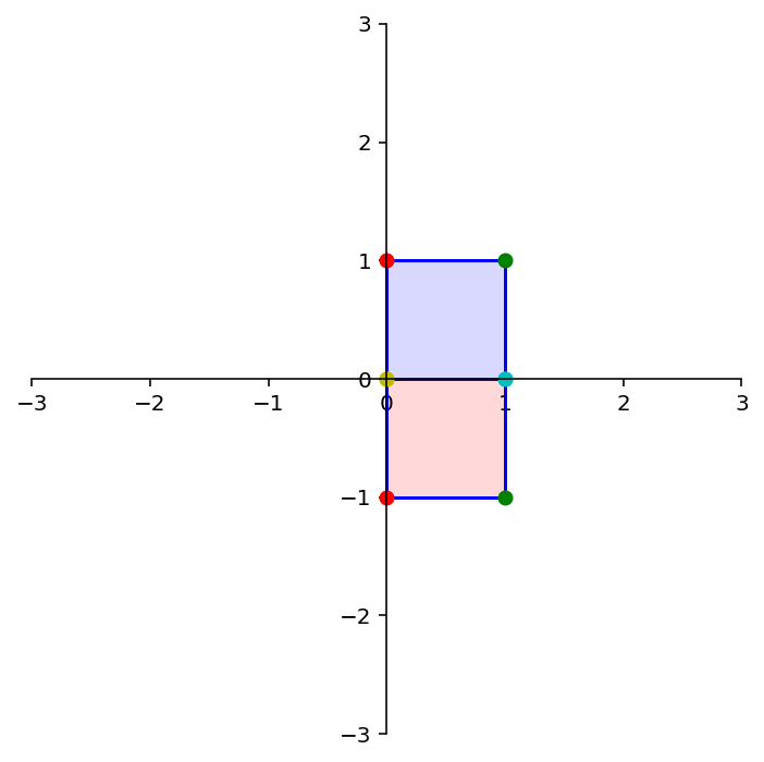
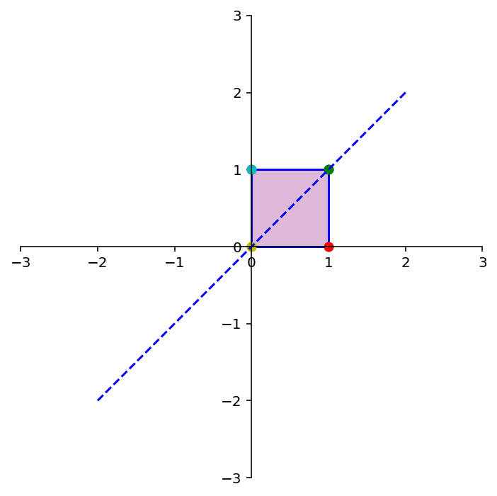
What about reflection through the line \(x_1 = x_2\)?
A = np.array(
    [[0,1],
     [1,0]])
print('A = \n',A)
dm.plotSetup()
dm.plotSquare(square)
dm.plotSquare(A @ square,'r')
plt.plot([-2,2],[-2,2],'b--')
Latex(r'Reflection through the line $x_1 = x_2$')
A =
 [[0 1]
 [1 0]]
dm.plotSetup()
dm.plotShape(note)
dm.plotShape(A @ note,'r')
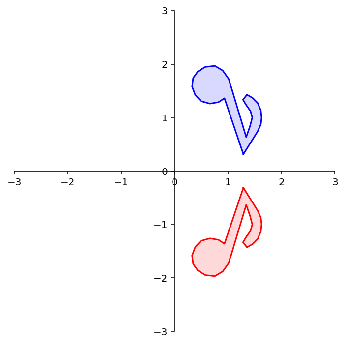
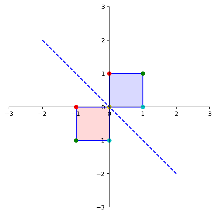
What about reflection through the line \(x_1 = -x_2\)?
A = np.array(
    [[ 0,-1],
     [-1, 0]])
print('A = \n',A)
dm.plotSetup()
dm.plotSquare(square)
dm.plotSquare(A @ square,'r')
plt.plot([-2,2],[2,-2],'b--')
Latex(r'Reflection through the line $x_1 = -x_2$')
A =
 [[ 0 -1]
 [-1  0]]
dm.plotSetup()
dm.plotShape(note)
dm.plotShape(A @ note,'r')

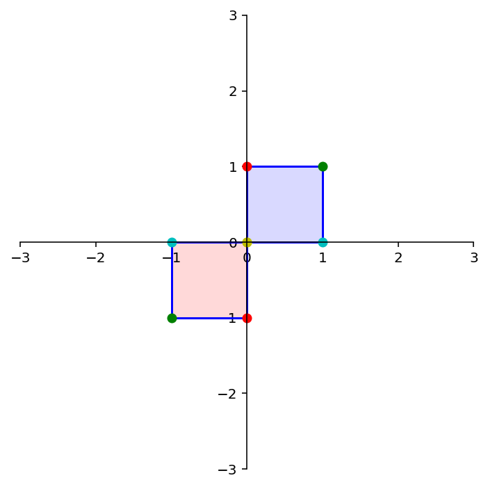
What about reflection through the origin?
A = np.array(
    [[-1, 0],
     [ 0,-1]])
print('A = \n',A)
ax = dm.plotSetup()
dm.plotSquare(square)
dm.plotSquare(A @ square,'r')
Latex(r'Reflection through the origin')
A =
 [[-1  0]
 [ 0 -1]]
dm.plotSetup()
dm.plotShape(note)
dm.plotShape(A @ note,'r')
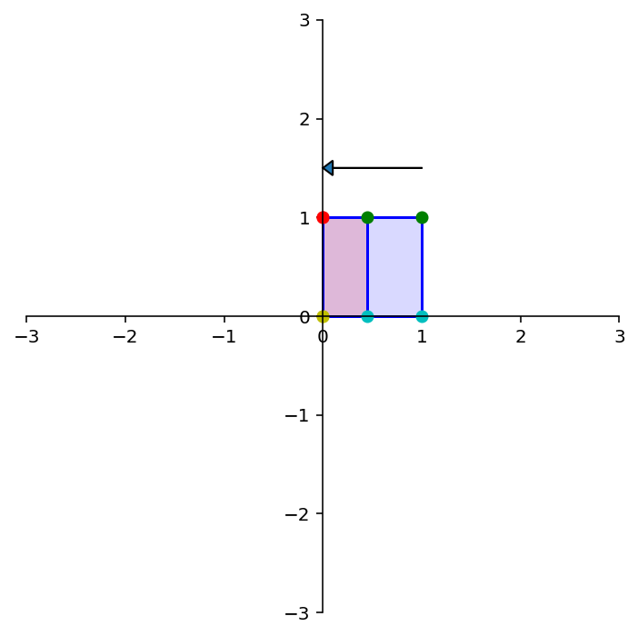
A = np.array(
    [[0.45, 0],
     [0,    1]])
print('A = \n',A)
ax = dm.plotSetup()
dm.plotSquare(square)
dm.plotSquare(A @ square,'r')
ax.arrow(1.0,1.5,-1.0,0,head_width=0.15, head_length=0.1, length_includes_head=True)
Latex(r'Horizontal Contraction')
A =
 [[0.45 0.  ]
 [0.   1.  ]]
dm.plotSetup()
dm.plotShape(note)
dm.plotShape(A @ note,'r')
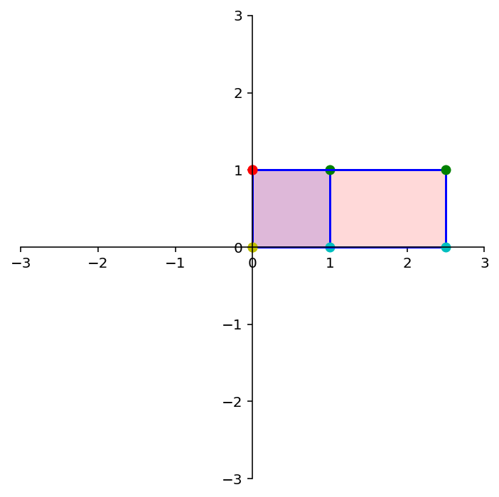
A = np.array(
    [[2.5,0],
     [0,  1]])
print('A = \n',A)
dm.plotSetup()
dm.plotSquare(square)
dm.plotSquare(A @ square,'r')
Latex(r'Horizontal Expansion')
A =
 [[2.5 0. ]
 [0.  1. ]]
A = np.array(
    [[   1, 0],
     [-1.5, 1]])
print('A = \n',A)
dm.plotSetup()
dm.plotSquare(square)
dm.plotSquare(A @ square,'r')
Latex(r'Vertical Shear')
A =
 [[ 1.   0. ]
 [-1.5  1. ]]
dm.plotSetup()
dm.plotShape(note)
dm.plotShape(A @ note,'r')

Question 8.2
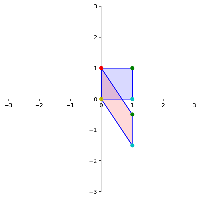
Now let’s look at a particular kind of transformation called a projection.
Imagine we took any given point and ‘dropped’ it onto the \(x_1\)-axis.
A = np.array(
    [[1,0],
     [0,0]])
print('A = \n',A)
ax = dm.plotSetup()
# dm.plotSquare(square)
dm.plotSquare(A @ square,'r')
ax.arrow(1.0,1.0,0,-0.9,head_width=0.15, head_length=0.1, length_includes_head=True)
ax.arrow(0.0,1.0,0,-0.9,head_width=0.15, head_length=0.1, length_includes_head=True)
Latex(r'Projection onto the $x_1$ axis')
A =
 [[1 0]
 [0 0]]
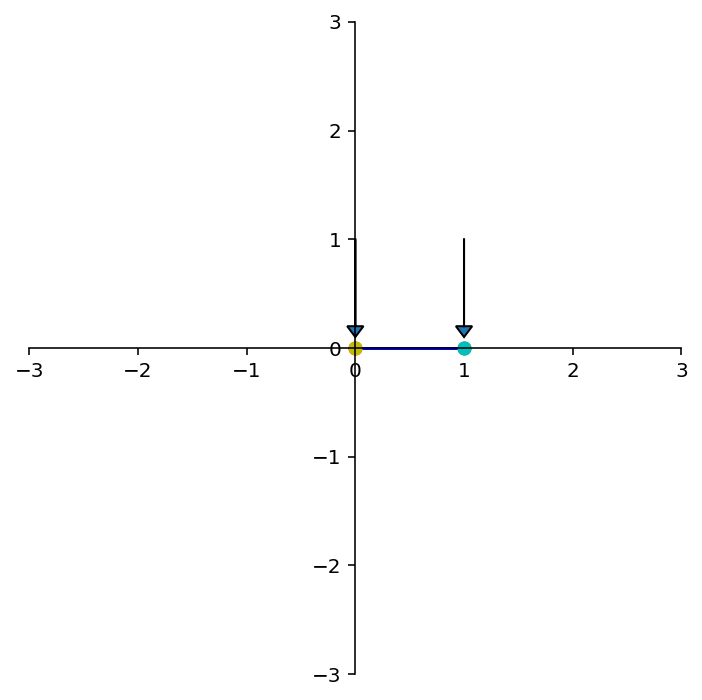
What happens to the shape of the point set?
dm.plotSetup()
dm.plotShape(note)
dm.plotShape(A @ note,'r')
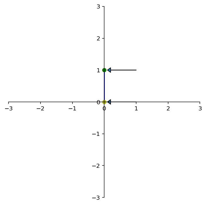
A = np.array(
    [[0,0],
     [0,1]])
print('A = \n',A)
ax = dm.plotSetup()
# dm.plotSquare(square)
dm.plotSquare(A @ square)
ax.arrow(1.0,1.0,-0.9,0,head_width=0.15, head_length=0.1, length_includes_head=True)
ax.arrow(1.0,0.0,-0.9,0,head_width=0.15, head_length=0.1, length_includes_head=True)
Latex(r'Projection onto the $x_2$ axis')
A =
 [[0 0]
 [0 1]]
dm.plotSetup()
dm.plotShape(note)
dm.plotShape(A @ note,'r')
Existence and Uniqueness
Notice that some of these transformations map multiple inputs to the same output, and some are incapable of generating certain outputs.
For example, the projections above can send multiple different points to the same point.
We need some terminology to understand these properties of linear transformations.
Definition. A mapping \(T: \mathbb{R}^n \rightarrow \mathbb{R}^m\) is said to be onto \(\mathbb{R}^m\) if each \(\mathbf{b}\) in \(\mathbb{R}^m\) is the image of at least one \(\mathbf{x}\) in \(\mathbb{R}^n\).
Informally, \(T\) is onto if every element of its codomain is in its range.
Another (important) way of thinking about this is that \(T\) is onto if there is a solution \(\mathbf{x}\) of
for all possible \(\mathbf{b}.\)
This is asking an existence question about a solution of the equation \(T(\mathbf{x}) = \mathbf{b}\) for all \(\mathbf{b}.\)
display(Image("images/L7 F4.jpg", width=650))
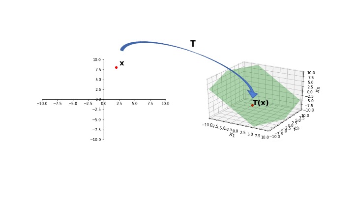
Here, we see that \(T\) maps points in \(\mathbb{R}^2\) to a plane lying within \(\mathbb{R}^3\).
That is, the range of \(T\) is a strict subset of the codomain of \(T\).
So \(T\) is not onto \(\mathbb{R}^3\).
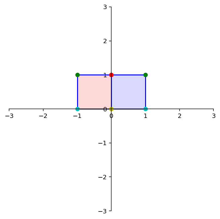
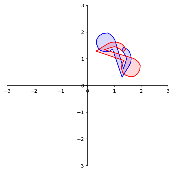
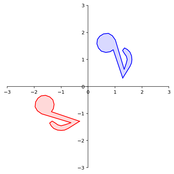
display(Image("images/L8 F3.png", width=650))
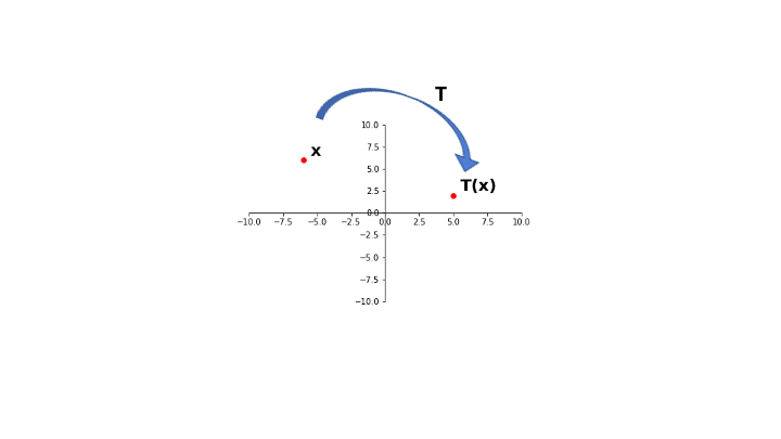
In this case, for every point in \(\mathbb{R}^2\), there is an \(\mathbf{x}\) that maps to that point.
So, the range of \(T\) is equal to the codomain of \(T\).
So \(T\) is onto \(\mathbb{R}^2\).
Here, the red points are the images of the blue points.
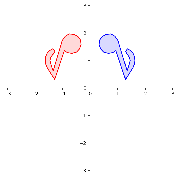
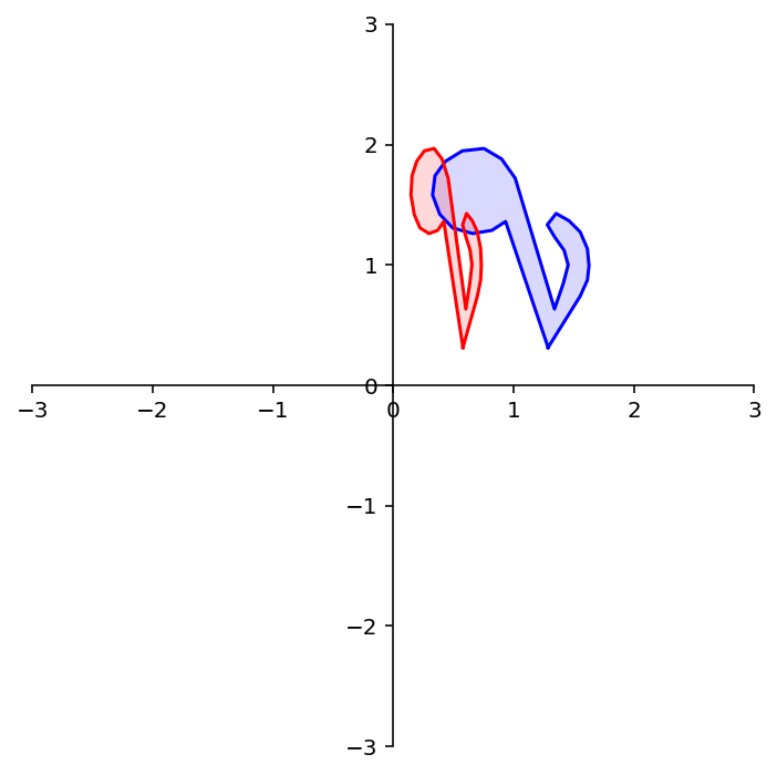
What about this transformation? Is it onto \(\mathbb{R}^2\)?
A = np.array(
    [[ 0,-1],
     [-1, 0]])
dm.plotSetup()
dm.plotShape(note)
dm.plotShape(A @ note,'r')
Here again the red points (which all lie on the \(x\)-axis) are the images of the blue points.
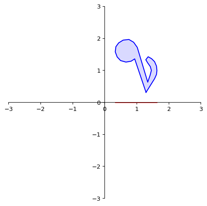
What about this transformation? Is it onto \(\mathbb{R}^2\)?
A = np.array(
    [[1,0],
     [0,0]])
dm.plotSetup()
dm.plotShape(note)
dm.plotShape(A @ note,'r')

Question Time! Q8.3
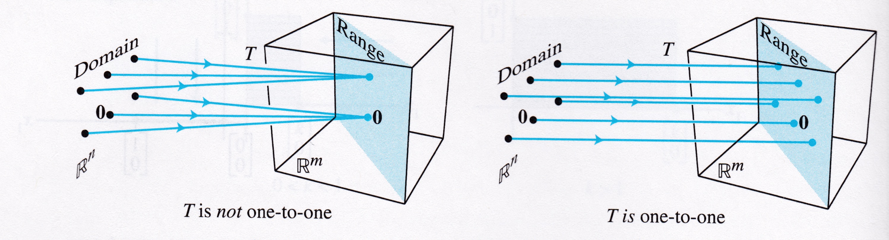
Definition. A mapping \(T: \mathbb{R}^n \rightarrow \mathbb{R}^m\) is said to be one-to-one if each \(\mathbf{b}\) in \(\mathbb{R}^m\) is the image of at most one \(\mathbf{x}\) in \(\mathbb{R}^n\).
If \(T\) is one-to-one, then for each \(\mathbf{b},\) the equation \(T(\mathbf{x}) = \mathbf{b}\) has either a unique solution, or none at all.
This is asking an existence question about a solution of the equation \(T(\mathbf{x}) = \mathbf{b}\) for all \(\mathbf{b}\).
# image credit: Lay, 4th edition
display(Image("images/Lay-fig-1-9-4.jpeg", width=650))
Let’s examine the relationship between these ideas and some previous definitions.
If \(A\mathbf{x} = \mathbf{b}\) is consistent for all \(\mathbf{b}\), is \(T(\mathbf{x}) = A\mathbf{x}\) onto? one-to-one?
\(T(\mathbf{x})\) is onto. \(T(\mathbf{x})\) may or may not be one-to-one. If the system has multiple solutions for some \(\mathbf{b}\), \(T(\mathbf{x})\) is not one-to-one.
If \(A\mathbf{x} = \mathbf{b}\) is consistent and has a unique solution for all \(\mathbf{b}\), is \(T(\mathbf{x}) = A\mathbf{x}\) onto? one-to-one?
Yes to both.
If \(A\mathbf{x} = \mathbf{b}\) is not consistent for all \(\mathbf{b}\), is \(T(\mathbf{x}) = A\mathbf{x}\) onto? one-to-one?
\(T(\mathbf{x})\) is not onto. \(T(\mathbf{x})\) may or may not be one-to-one.
If \(T(\mathbf{x}) = A\mathbf{x}\) is onto, is \(A\mathbf{x} = \mathbf{b}\) consistent for all \(\mathbf{b}\)? is the solution unique for all \(\mathbf{b}\)?
If \(T(\mathbf{x}) = A\mathbf{x}\) is one-to-one, is \(A\mathbf{x} = \mathbf{b}\) consistent for all \(\mathbf{b}\)? is the solution unique for all \(\mathbf{b}\)?