# for QR codes use inline
%matplotlib inline
qr_setting = None
#
# for lecture use notebook
# %matplotlib notebook
# qr_setting = None
#
%config InlineBackend.figure_format='retina'
# import libraries
import numpy as np
import matplotlib as mp
import pandas as pd
import matplotlib.pyplot as plt
import laUtilities as ut
import slideUtilities as sl
import demoUtilities as dm
import pandas as pd
from importlib import reload
from datetime import datetime
from IPython.display import Image
from IPython.display import display_html
from IPython.display import display
from IPython.display import Math
from IPython.display import Latex
from IPython.display import HTML;
Subspaces
fig = ut.three_d_figure((0,0), fig_desc = 'H = Span{a1, a2, a3}',
                        xmin = -10, xmax = 10, ymin = -10, ymax = 10, zmin = -10, zmax = 10, qr = qr_setting)
a1 = [-8.0, 8.0, 5.0]
a2 = [3.0,  2.0, -2.0]
a3 = 2.5 * np.array(a2)
fig.text(a1[0]+.5, a1[1]+.5, a1[2]+.5, r'$\bf a_1$', 'a_1', size=18)
fig.text(a3[0]+.5, a3[1]+.5, a3[2]+.5, r'$\bf a_3$', 'a_3', size=18)
fig.text(a2[0]+.5, a2[1]+.5, a2[2]+.5, r'$\bf a_2$', 'a_2', size=18)
fig.plotSpan(a1, a2,'Green')
fig.plotPoint(a1[0], a1[1], a1[2],'r')
fig.plotPoint(a3[0], a3[1], a3[2],'r')
fig.plotPoint(a2[0], a2[1], a2[2],'r')
fig.plotLine([[0, 0, 0], a3], 'r', '--')
fig.plotLine([[0, 0, 0], a1], 'r', '--')
# fig.plotPoint(a3[0], a3[1], a3[2],'r')
fig.text(0.1, 0.1, -3, r'$\bf 0$', '0', size=12)
fig.plotPoint(0, 0, 0, 'b')
# fig.set_title(r'$H$ = Span$\{{\bf a}_1, {\bf a}_2, {\bf a}_3\}$')
fig.text(9, -9, -7, r'H', 'H', size = 16)
img = fig.dont_save()
Where we’ve been and where we’re going
We are at the midpoint of the course.
We’ve done a lot.
We started from the idea of solving linear systems.
From there, we’ve developed an algebra of matrices and vectors.
This has led us to a view of a matrix as a linear operator: something that acts on a vector to create a new vector.
We’ve seen how this view leads to insight into various problems, including problems related to
Flow balance,
Markov chains, and
computer graphics.
Here is where we’re headed:
This week: foundations for what’s ahead
Subspace, Basis, and Dimension
Then two weeks on Eigenvalues and Eigenvectors
Applications: dynamical systems, random walks, and Google PageRank
Then two weeks on Analytic Geometry
Applications:
Solving inconsistent linear systems (Least squares)
Machine learning: linear models
Then one week on Symmetric Matrices
Applications: Optimization and Data Mining
… let’s get started!
Subspaces
So far have been working with vector spaces like \(\mathbb{R}^2, \mathbb{R}^3.\)
But there are more vector spaces…
Today we’ll define a subspace and show how the concept helps us understand the nature of matrices and their linear transformations.
Definition. A subspace is any set \(H\) in \(\mathbb{R}^n\) that has three properties:
The zero vector is in \(H\).
For each \(\mathbf{u}\) and \(\mathbf{v}\) in \(H\), the sum \(\mathbf{u} + \mathbf{v}\) is in \(H\).
For each \(\mathbf{u}\) in \(H\) and each scalar \(c,\) the vector \(c\mathbf{u}\) is in \(H\).
Another way of stating properties 2 and 3 is that \(H\) is closed under addition and scalar multiplication.
Every Span is a Subspace
The first thing to note is that there is a close connection between Span and Subspace:
To see this, let’s take a specific example.
For example, take \(\mathbf{v}_1\) and \(\mathbf{v}_2\) in \(\mathbb{R}^n\), and let \(H\) = Span\(\{\mathbf{v}_1, \mathbf{v}_2\}.\)
Then \(H\) is a subspace of \(\mathbb{R}^n\).
fig = ut.three_d_figure((14, 1), fig_desc = 'Span{v1, v2}, a subspace.',
                        xmin = -10, xmax = 10, ymin = -10, ymax = 10, zmin = -10, zmax = 10, qr = qr_setting)
a1 = [-8.0, 8.0, 5.0]
a2 = [3.0,  2.0, -2.0]
a3 = 2.5 * np.array(a2)
fig.text(a1[0]+.5, a1[1]+.5, a1[2]+.5, r'$\bf v_1$', 'v_1', size=20)
fig.text(a3[0]+.5, a3[1]+.5, a3[2]+.5, r'$\bf v_2$', 'v_2', size=20)
fig.plotSpan(a1, a2,'Green')
fig.plotPoint(a1[0], a1[1], a1[2],'r')
fig.plotPoint(a3[0], a3[1], a3[2],'r')
# fig.plotPoint(a3[0], a3[1], a3[2],'r')
#fig.text(a1[0], a1[1], a1[2], r'$\bf v_1$', 'a_1', size=20)
fig.text(0.1, 0.1, -3, r'$\bf 0$', '0', size=12)
fig.plotPoint(0, 0, 0, 'b')
fig.set_title(r'Span{$v_1, v_2$}, a subspace.')
fig.text(9, -9, -7, r'$\bf H$', 'H', size = 20)
img = fig.save()
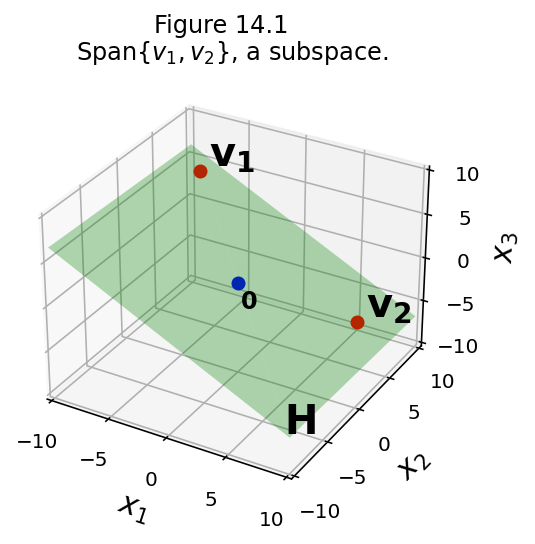
Let’s check this:
The zero vector is in \(H\)
…because \({\bf 0} = 0\mathbf{v}_1 + 0\mathbf{v}_2\) is in Span\(\{\mathbf{v}_1, \mathbf{v}_2\}.\)
The sum of any two vectors in \(H\) is in \(H\)
In other words, if \(\mathbf{u} = s_1\mathbf{v}_1 + s_2\mathbf{v}_2,\) and \(\mathbf{v} = t_1\mathbf{v}_1 + t_2\mathbf{v}_2,\)
…their sum \(\mathbf{u} + \mathbf{v}\) is \((s_1+t_1)\mathbf{v}_1 + (s_2+t_2)\mathbf{v}_2,\)
…which is in \(H\).
For any scalar \(c\), \(c\mathbf{u}\) is in \(H\)
because \(c\mathbf{u} = c(s_1\mathbf{v}_1 + s_2\mathbf{v}_2) = (cs_1\mathbf{v}_1 + cs_2\mathbf{v}_2).\)
Because of this, we refer to Span\(\{\mathbf{v}_1,\dots,\mathbf{v}_p\}\) as the subspace spanned by \(\mathbf{v}_1,\dots,\mathbf{v}_p.\)
OK, here is another subspace – a line:
fig = ut.three_d_figure((14, 2), fig_desc = 'Span{v1}, another subspace.',
                        xmin = -10, xmax = 10, ymin = -10, ymax = 10, zmin = -10, zmax = 10, qr = qr_setting)
v = [ 4.0, 4.0, 2.0]
fig.text(v[0]+.5, v[1]+.5, v[2]+.5, r'$\bf v_1$', 'v1', size=20)
fig.text(-9, -7, -9, r'Span{$\bf v_1$}', 'Span{v1}', size=16)
fig.text(0.2, 0.2, -4, r'$\bf 0$', '0', size=12)
# plotting the span of v
# this is based on the reduced echelon matrix that expresses the system whose solution is v
fig.plotIntersection([1, 0, -v[0]/v[2], 0], [0, 1, -v[1]/v[2], 0], '-', 'Red')
fig.plotPoint(v[0], v[1], v[2], 'r')
fig.plotPoint(0, 0, 0, 'b')
# plotting the axes
fig.plotIntersection([0, 0, 1, 0], [0, 1, 0, 0])
fig.plotIntersection([0, 0, 1, 0], [1, 0, 0, 0])
fig.plotIntersection([0, 1, 0, 0], [1, 0, 0, 0])
fig.set_title(r'Span {$v_1$}, another subspace.')
img = fig.save()
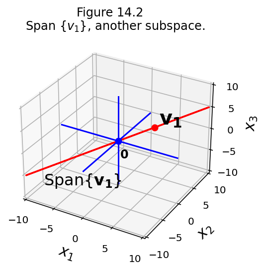
Next question: is any line a subspace?
What about a line that is not through the origin?
How about this line:
ax = ut.plotSetup()
ut.centerAxes(ax)
ax.plot([-6,6],[4.33,0.33],'b-')
ax.text(-4,3,'$L$',size=20);
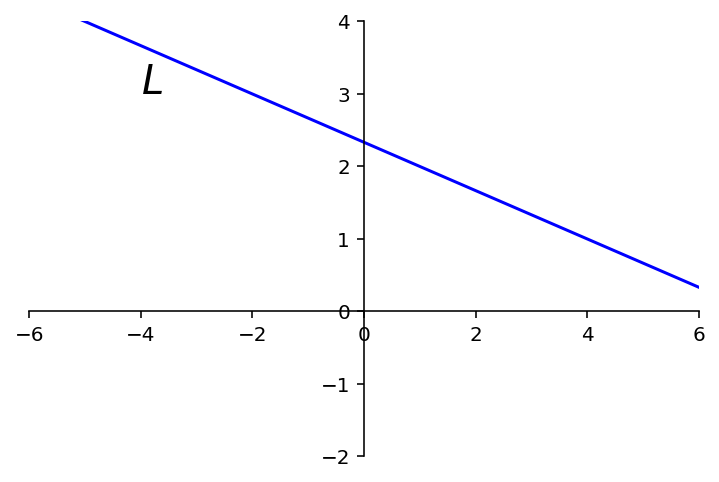
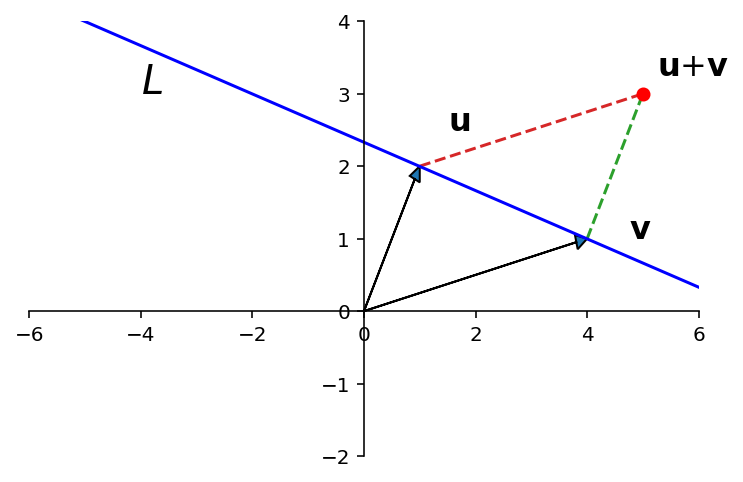
In fact, a line \(L\) not through the origin fails all three requirements for a subspace:
\(L\) does not contain the zero vector.
\(L\) is not closed under addition.
ax = ut.plotSetup()
ut.centerAxes(ax)
ax.arrow(0,0,1,2,head_width=0.2, head_length=0.2,length_includes_head = True)
ax.arrow(0,0,4,1,head_width=0.2, head_length=0.2,length_includes_head = True)
ax.plot([4,5],[1,3],'--')
ax.plot([1,5],[2,3],'--')
ax.plot([-6,6],[4.33,0.33],'b-')
ax.text(5.25,3.25,r'${\bf u}$+${\bf v}$',size=16)
ax.text(1.5,2.5,r'${\bf u}$',size=16)
ax.text(4.75,1,r'${\bf v}$',size=16)
ax.text(-4,3,'$L$',size=20)
ut.plotPoint(ax,5,3)
ax.plot(0,0,'');
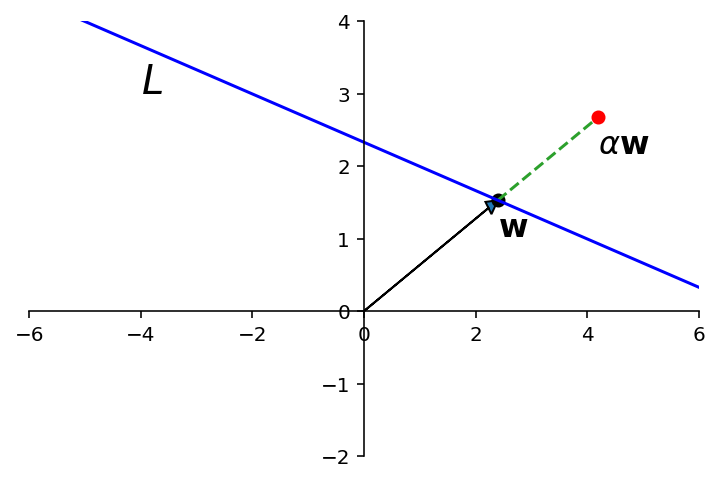
\(L\) is not closed under scalar multiplication.
ax = ut.plotSetup()
ut.centerAxes(ax)
line = np.array([[-6,6],[4.33,0.33]])
w = .3 * line[:,0] + .7 * line[:,1]
ut.plotPoint(ax,w[0],w[1],'k')
ax.arrow(0,0,w[0],w[1],head_width=0.2, head_length=0.2,length_includes_head = True)
w_ext = np.array([w, 1.75*w]).T
ax.plot(w_ext[0], w_ext[1], '--')
ax.plot(line[0], line[1],'b-')
ax.text(w[0],w[1]-0.5,r'${\bf w}$',size=16)
ax.text(w_ext[0,1], w_ext[1,1]-0.5, r'$\alpha{\bf w}$', size=16)
ut.plotPoint(ax,w_ext[0,1],w_ext[1,1],'r')
ax.text(-4,3,'$L$',size=20);
On the other hand, any line, plane, or hyperplane through the origin is a subspace.
Make sure you can see why (or prove it to yourself).
Question Time! Q14.1
Two Important Subspaces
Now let’s start to use the subspace concept to characterize matrices.
We are thinking of these matrices as linear operators.
Every matrix has associated with it two subspaces:
column space and
null space.
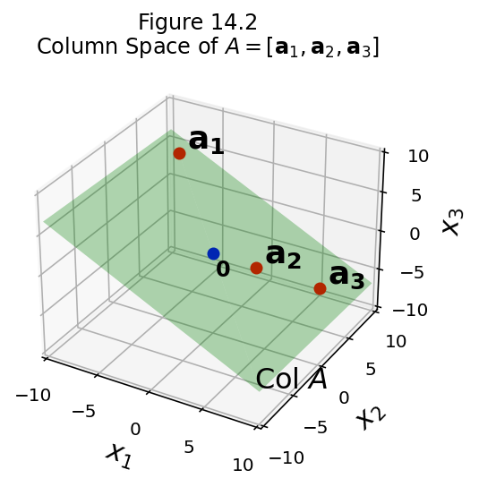
Column Space
Definition. The column space of a matrix \(A\) is the set \({\operatorname{Col}}\ A\) of all linear combinations of the columns of \(A\).
If \(A\) = \([\mathbf{a}_1 \;\cdots\; \mathbf{a}_n]\), with columns in \(\mathbb{R}^m,\) then \({\operatorname{Col}}\ A\) is the same as Span\(\{\mathbf{a}_1,\dots,\mathbf{a}_n\}.\)
The column space of an \(m\times n\) matrix is a subspace of \(\mathbb{R}^m.\)
In particular, note that \({\operatorname{Col}}\ A\) equals \(\mathbb{R}^m\) only when the columns of \(A\) span \(\mathbb{R}^m.\)
Otherwise, \({\operatorname{Col}}\ A\) is only part of \(\mathbb{R}^m.\)
When a system of linear equations is written in the form \(A\mathbf{x} = \mathbf{b},\) the column space of \(A\) is the set of all \(\mathbf{b}\) for which the system has a solution.
Equivalently, when we consider the linear operator \(T: \mathbb{R}^n\rightarrow\mathbb{R}^m\) that is implemented by the matrix \(A\), the column space of \(A\) is the range of \(T.\)
fig = ut.three_d_figure((14, 2), fig_desc = 'Column Space of A = [a1, a2, a3].',
                        xmin = -10, xmax = 10, ymin = -10, ymax = 10, zmin = -10, zmax = 10, qr = qr_setting)
a1 = [-8.0, 8.0, 5.0]
a2 = [3.0,  2.0, -2.0]
a3 = 2.5 * np.array(a2)
fig.text(a1[0]+.5, a1[1]+.5, a1[2]+.5, r'$\bf a_1$', 'a_1', size=18)
fig.text(a3[0]+.5, a3[1]+.5, a3[2]+.5, r'$\bf a_3$', 'a_3', size=18)
fig.text(a2[0]+.5, a2[1]+.5, a2[2]+.5, r'$\bf a_2$', 'a_2', size=18)
fig.plotSpan(a1, a2,'Green')
fig.plotPoint(a1[0], a1[1], a1[2],'r')
fig.plotPoint(a3[0], a3[1], a3[2],'r')
fig.plotPoint(a2[0], a2[1], a2[2],'r')
# fig.plotPoint(a3[0], a3[1], a3[2],'r')
fig.text(0.1, 0.1, -3, r'$\bf 0$', '0', size=12)
fig.plotPoint(0, 0, 0, 'b')
fig.set_title(r'Column Space of $A = [{\bf a}_1, {\bf a}_2, {\bf a}_3]$')
fig.text(9, -9, -7, r'Col $A$', 'H', size = 16)
img = fig.save()
Question Time! Q14.2
Null Space
Definition. The null space of a matrix \(A\) is the set \({\operatorname{Nul}}\ A\) of all solutions of the homogeneous equation \(A\mathbf{x} = 0.\)
In other words: the null space of \(A\) is the set of all vectors that are mapped to the zero vector by \(A\).
When \(A\) has \(n\) columns, a solution of \(A\mathbf{x} = {\bf 0}\) is a vector in \(\mathbb{R}^n.\) So the null space of \(A\) is a subset of \(\mathbb{R}^n.\)
In fact, \({\operatorname{Nul}}\ A\) is a subspace of \(\mathbb{R}^n.\)
Theorem. The null space of an \(m\times n\) matrix \(A\) is a subspace of \(\mathbb{R}^n.\)
Equivalently, the set of all solutions of a system \(A\mathbf{x} = {\bf 0}\) of \(m\) homogeneous linear equations in \(n\) unknowns is a subspace of \(\mathbb{R}^n.\)
Proof.
The zero vector is in \({\operatorname{Nul}}\ A\) because \(A{\bf 0} = {\bf 0}.\)
The sum of two vectors in \({\operatorname{Nul}}\ A\) is in \({\operatorname{Nul}}\ A.\)
Take two vectors \(\mathbf{u}\) and \(\mathbf{v}\) that are in \({\operatorname{Nul}}\ A.\) By definition \(A\mathbf{u} = {\bf 0}\) and \(A\mathbf{v} = {\bf 0}.\)
Then \(\mathbf{u} + \mathbf{v}\) is in \({\operatorname{Nul}}\ A\) because \(A(\mathbf{u} + \mathbf{v}) = A\mathbf{u} + A\mathbf{v} = {\bf 0} + {\bf 0} = {\bf 0}.\)
Any scalar multiple of a vector in \({\operatorname{Nul}}\ A\) is in \({\operatorname{Nul}}\ A.\)
Take a vector \(\mathbf{v}\) that is in \({\operatorname{Nul}}\ A.\) Then \(A(c\mathbf{v}) = cA\mathbf{v} = c{\bf 0} = {\bf 0}.\)
Testing whether a vector \(\mathbf{v}\) is in \({\operatorname{Nul}}\ A\) is easy: simply compute \(A\mathbf{v}\) and see if the result is zero.
Comparing \({\operatorname{Col}}\ A\) and \({\operatorname{Nul}}\ A\).
What is the relationship between these two subspaces that are defined using \(A\)?
Actually, there is no particular connection (at this moment in the course).
The important thing to note at present is that these two subspaces live in different “universes”.
For an \(m\times n\) matrix,
the column space is a subset of \(\mathbb{R}^m\) (all its vectors have \(m\) components),
while the null space is a subset of \(\mathbb{R}^n\) (all its vectors have \(n\) components).
However: next lecture we will make a connection!
A Basis for a Subspace
Let’s say you have a subspace.
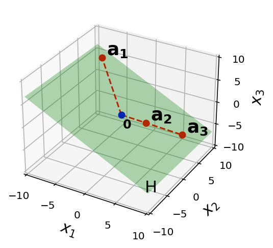
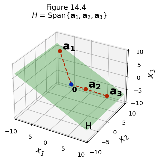
For example, perhaps it is Span\(\{\mathbf{a}_1, \mathbf{a}_2, \mathbf{a}_3\}\).
We would like to find the simplest way of describing this space.
For example, consider this subspace:
fig = ut.three_d_figure((14, 3), fig_desc = 'H = Span{a1, a2, a3}',
                        xmin = -10, xmax = 10, ymin = -10, ymax = 10, zmin = -10, zmax = 10, qr = qr_setting)
a1 = [-8.0, 8.0, 5.0]
a2 = [3.0,  2.0, -2.0]
a3 = 2.5 * np.array(a2)
fig.text(a1[0]+.5, a1[1]+.5, a1[2]+.5, r'$\bf a_1$', 'a_1', size=18)
fig.text(a3[0]+.5, a3[1]+.5, a3[2]+.5, r'$\bf a_3$', 'a_3', size=18)
fig.text(a2[0]+.5, a2[1]+.5, a2[2]+.5, r'$\bf a_2$', 'a_2', size=18)
fig.plotSpan(a1, a2,'Green')
fig.plotPoint(a1[0], a1[1], a1[2],'r')
fig.plotPoint(a3[0], a3[1], a3[2],'r')
fig.plotPoint(a2[0], a2[1], a2[2],'r')
# fig.plotPoint(a3[0], a3[1], a3[2],'r')
fig.text(0.1, 0.1, -3, r'$\bf 0$', '0', size=12)
fig.plotPoint(0, 0, 0, 'b')
fig.set_title(r'$H$ = Span$\{{\bf a}_1, {\bf a}_2, {\bf a}_3\}$')
fig.text(9, -9, -7, r'H', 'H', size = 16)
img = fig.save()
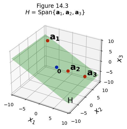
Note that \(\mathbf{a}_3\) is a scalar multiple of \(\mathbf{a}_2\). Thus:
Span\(\{\mathbf{a}_1, \mathbf{a}_2, \mathbf{a}_3\}\)
is the same subspace as
Span\(\{\mathbf{a}_1, \mathbf{a}_2\}\).
Can you see why?
fig = ut.three_d_figure((14, 4), fig_desc = 'H = Span{a1, a2, a3}',
                        xmin = -10, xmax = 10, ymin = -10, ymax = 10, zmin = -10, zmax = 10, qr = qr_setting)
a1 = [-8.0, 8.0, 5.0]
a2 = [3.0,  2.0, -2.0]
a3 = 2.5 * np.array(a2)
fig.text(a1[0]+.5, a1[1]+.5, a1[2]+.5, r'$\bf a_1$', 'a_1', size=18)
fig.text(a3[0]+.5, a3[1]+.5, a3[2]+.5, r'$\bf a_3$', 'a_3', size=18)
fig.text(a2[0]+.5, a2[1]+.5, a2[2]+.5, r'$\bf a_2$', 'a_2', size=18)
fig.plotSpan(a1, a2,'Green')
fig.plotPoint(a1[0], a1[1], a1[2],'r')
fig.plotPoint(a3[0], a3[1], a3[2],'r')
fig.plotPoint(a2[0], a2[1], a2[2],'r')
fig.plotLine([[0, 0, 0], a3], 'r', '--')
fig.plotLine([[0, 0, 0], a1], 'r', '--')
# fig.plotPoint(a3[0], a3[1], a3[2],'r')
fig.text(0.1, 0.1, -3, r'$\bf 0$', '0', size=12)
fig.plotPoint(0, 0, 0, 'b')
fig.set_title(r'$H$ = Span$\{{\bf a}_1, {\bf a}_2, {\bf a}_3\}$')
fig.text(9, -9, -7, r'H', 'H', size = 16)
img = fig.save()
Making this idea more general:
we would like to describe a subspace as the span of a set of vectors, and
that set of vectors should have the fewest members as possible!
So in our example above, we would prefer to say that the subspace is:
\(H\) = Span\(\{\mathbf{a}_1, \mathbf{a}_2\}\)
rather than
\(H\) = Span\(\{\mathbf{a}_1, \mathbf{a}_2, \mathbf{a}_3\}\).
In other words, the more “concisely” we can describe the subspace, the better.
Now, given some subspace, how small a spanning set can we find?
Here is the key idea we will use to answer that question:
It can be shown that the smallest possible spanning set must be linearly independent.
We will call such minimally-small sets of vectors a basis for the space.
Definition. A basis for a subspace \(H\) of \(\mathbb{R}^n\) is a linearly independent set in \(H\) that spans \(H.\)
fig = ut.three_d_figure((14, 5), fig_desc = 'Bases of H are {a1, a2} or {a1, a3}.',
                        xmin = -10, xmax = 10, ymin = -10, ymax = 10, zmin = -10, zmax = 10, qr = qr_setting)
a1 = [-8.0, 8.0, 5.0]
a2 = [3.0,  2.0, -2.0]
a3 = 2.5 * np.array(a2)
fig.text(a1[0]+.5, a1[1]+.5, a1[2]+.5, r'$\bf a_1$', 'a_1', size=18)
fig.text(a3[0]+.5, a3[1]+.5, a3[2]+.5, r'$\bf a_3$', 'a_3', size=18)
fig.text(a2[0]+.5, a2[1]+.5, a2[2]+.5, r'$\bf a_2$', 'a_2', size=18)
fig.plotSpan(a1, a2,'Green')
fig.plotPoint(a1[0], a1[1], a1[2],'r')
fig.plotPoint(a3[0], a3[1], a3[2],'r')
fig.plotPoint(a2[0], a2[1], a2[2],'r')
fig.plotLine([[0, 0, 0], a3], 'r', '--')
fig.plotLine([[0, 0, 0], a1], 'r', '--')
# fig.plotPoint(a3[0], a3[1], a3[2],'r')
fig.text(0.1, 0.1, -3, r'$\bf 0$', '0', size=12)
fig.plotPoint(0, 0, 0, 'b')
fig.set_title(r'Bases of $H$ are $\{{\bf a}_1, {\bf a}_2\}$ or $\{{\bf a}_1, {\bf a}_3\}$')
fig.text(9, -9, -7, r'H', 'H', size = 16)
img = fig.save()
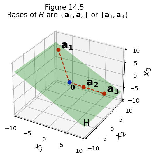
So in the example above, a basis for \(H\) could be:
\(\{\mathbf{a}_1, \mathbf{a}_2\}\)
or
\(\{\mathbf{a}_1, \mathbf{a}_3\}.\)
However,
\(\{\mathbf{a}_1, \mathbf{a}_2, \mathbf{a}_3\}\)
is not a basis for \(H\).
That is because \(\{\mathbf{a}_1, \mathbf{a}_2, \mathbf{a}_3\}\) are not linearly independent.
(Conceptually, there are “too many vectors” in this set).
And furthermore,
\(\{\mathbf{a}_1\}\)
is not a basis for \(H\).
That is because \(\{\mathbf{a}_1\}\) does not span \(H\).
(Conceptually, there are “not enough vectors” in this set).
Example.
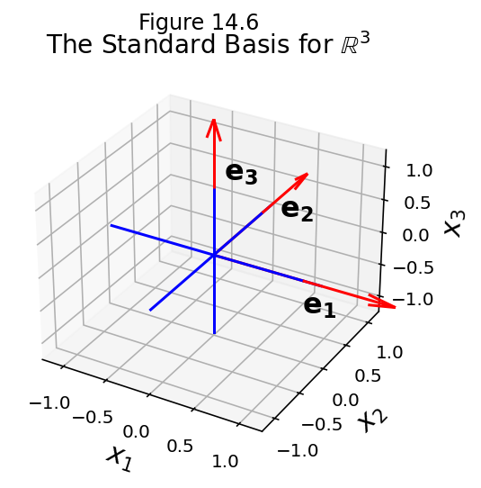
The columns of any invertible \(n\times n\) matrix form a basis for \(\mathbb{R}^n.\)
This is because, by the Invertible Matrix Theorem, they are linearly independent, and they span \(\mathbb{R}^n.\)
So, for example, we could use the identity matrix, \(I.\) It columns are \(\mathbf{e}_1, \dots, \mathbf{e}_n.\)
The set \(\{\mathbf{e}_1,\dots,\mathbf{e}_n\}\) is called the standard basis for \(\mathbb{R}^n.\)
fig = ut.three_d_figure((14, 6), fig_desc = 'The Standard Basis for R3',
                        xmin = -1.2, xmax = 1.2, ymin = -1.2, ymax = 1.2, zmin = -1.2, zmax = 1.2, qr = qr_setting)
e1 = [1, 0, 0]
e2 = [0, 1, 0]
e3 = [0, 0, 1]
origin = [0, 0, 0]
fig.ax.quiver(e1, e2, e3, e1, e2, e3, length=1.0, color='Red')
fig.plotLine([[0, 0, 0], [0, 1, 0]], color='Red')
fig.plotLine([[0, 0, 0], [0, 0, 1]], color='Red')
fig.plotLine([[0, 0, 0], [1, 0, 0]], color='Red')
fig.text(1, 0, -0.5, r'${\bf e_1}$', 'e1', size=16)
fig.text(0.2, 1, 0, r'${\bf e_2}$', 'e2', size=16)
fig.text(0, 0.2, 1, r'${\bf e_3}$', 'e3', size=16)
# plotting the axes
fig.plotIntersection([0, 0, 1, 0], [0, 1, 0, 0])
fig.plotIntersection([0, 0, 1, 0], [1, 0, 0, 0])
fig.plotIntersection([0, 1, 0, 0], [1, 0, 0, 0])
fig.set_title(r'The Standard Basis for $\mathbb{R}^3$',size=14);
fig.save();
Question Time! Q14.3
Bases for Null and Column Spaces
Being able to express a subspace in terms of a basis is very powerful.
It gives us a concise way of describing the subspace.
And we will see in the next lecture, that it will allow us to introduce ideas of coordinate systems and dimension.
Hence, we will often want to be able to describe subspaces like \(\operatorname{Col} A\) or \(\operatorname{Nul} A\) using their bases.
Finding a basis for the Null Space
We’ll start with finding a basis for the null space of a matrix.
Example. Find a basis for the null space of the matrix
Solution. We would like to describe the set of all solutions of \(A\mathbf{x} = {\bf 0}.\)
We start by writing the solution of \(A\mathbf{x} = {\bf 0}\) in parametric form:
So \(x_1\) and \(x_3\) are basic, and \(x_2, x_4,\) and \(x_5\) are free.
So the general solution is:
Now, what we want to do is write the solution set as a weighted combination of vectors.
This is a neat trick – we are creating a vector equation.
The key idea is that the free variables will become the weights.
Now what we have is an expression that describes the entire solution set of \(A\mathbf{x} = {\bf 0}.\)
So \({\operatorname{Nul}}\ A\) is the set of all linear combinations of \(\mathbf{u}, \mathbf{v},\) and \({\bf w}\). That is, \({\operatorname{Nul}}\ A\) is the subspace spanned by \(\{\mathbf{u}, \mathbf{v}, {\bf w}\}.\)
Furthermore, this construction automatically makes \(\mathbf{u}, \mathbf{v},\) and \({\bf w}\) linearly independent.
Since each weight appears by itself in one position, the only way for the whole weighted sum to be zero is if every weight is zero – which is the definition of linear independence.
So \(\{\mathbf{u}, \mathbf{v}, {\bf w}\}\) is a basis for \({\operatorname{Nul}}\ A.\)
Conclusion: by finding a parametric description of the solution of the equation \(A\mathbf{x} = {\bf 0},\) we can construct a basis for the nullspace of \(A\).
Finding a basis for the Column Space
To find a basis for the column space, we have an easier starting point.
We know that the column space is the span of the matrix columns.
So, we can choose matrix columns to make up the basis.
The question is: which columns should we choose?
Warmup.
We start with a warmup example.
Suppose we have a matrix \(B\) that happens to be in reduced echelon form:
Denote the columns of \(B\) by \(\mathbf{b}_1,\dots,\mathbf{b}_5\).
Note that \(\mathbf{b}_3 = -3\mathbf{b}_1 + 2\mathbf{b}_2\) and \(\mathbf{b}_4 = 5\mathbf{b}_1-\mathbf{b}_2.\)
So any combination of \(\mathbf{b}_1,\dots,\mathbf{b}_5\) is actually just a combination of \(\mathbf{b}_1, \mathbf{b}_2,\) and \(\mathbf{b}_5.\)
So \(\{\mathbf{b}_1, \mathbf{b}_2, \mathbf{b}_5\}\) spans \({\operatorname{Col}}\ B\).
Also, \(\mathbf{b}_1, \mathbf{b}_2,\) and \(\mathbf{b}_5\) are linearly independent, because they are columns from an identity matrix.
So: the pivot columns of \(B\) form a basis for \({\operatorname{Col}}\ B.\)
Note that this means: there is no combination of columns 1, 2, and 5 that yields the zero vector.
(Other than the trivial combination of course.)
So, for matrices in reduced row echelon form, we have a simple rule for the basis of the column space:
Choose the columns that hold the pivots.
The general case.
Now I’ll show that the pivot columns of \(A\) form a basis for \({\operatorname{Col}}\ A\) for any \(A\).
Consider the case where \(A\mathbf{x} = {\bf 0}\) for some nonzero \(\mathbf{x}.\)
This says that there is a linear dependence relation between some of the columns of \(A\).
If any of the entries in \(\mathbf{x}\) are zero, then those columns do not participate in the linear dependence relation.
When we row-reduce \(A\) to its reduced echelon form \(B\), the columns are changed, but the equations \(A\mathbf{x} = {\bf 0}\) and \(B\mathbf{x} = {\bf 0}\) have the same solution set.
So this means that the columns of \(A\) and the columns of \(B\) have exactly the same dependence relationships as the columns of \(B\).
In other words:
If some column of \(B\) can be written as a combination of other columns of \(B\), then the same is true of the corresponding columns of \(A\).
If no combination of certain columns of \(B\) yields the zero vector, then no combination of corresponding columns of \(A\) yields the zero vector.
In other words:
If some set of columns of \(B\) spans the column space of \(B\), then the same columns of \(A\) span the column space of \(A\).
If some set of columns of \(B\) are linearly independent, then the same columns of \(A\) are linearly independent.
So, if some columns of \(B\) are a basis for \({\operatorname{Col}}\ B\), then the corresponding columns of \(A\) are a basis for \({\operatorname{Col}}\ A\).
Example. Consider the matrix \(A\):
It is row equivalent to the matrix \(B\) that we considered above. So to find its basis, we simply need to look at the basis for its reduced row echelon form. We already computed that a basis for \({\operatorname{Col}}\ B\) was columns 1, 2, and 5.
Therefore we can immediately conclude that a basis for \({\operatorname{Col}}\ A\) is \(A\)’s columns 1, 2, and 5.
So a basis for \({\operatorname{Col}}\ A\) is:
Theorem. The pivot columns of a matrix \(A\) form a basis for the column space of \(A\).
Be careful here – note that we compute the reduced row echelon form of \(A\) to find which columns are pivot columns…
but we use the columns of \(A\) itself as the basis for \({\operatorname{Col}}\ A\)!