The Characteristic Equation¶

A = np.array([[0.8, 0.5],[-0.1, 1.0]])

x =  np.array([1,500.])
fig = plt.figure()
ax = plt.axes(xlim=(-500,500),ylim=(-500,500))
plt.plot(-500, -500,''),
plt.plot(500, 500,'')
plt.axis('equal')
for i in range(75):
    newx = A @ x
    plt.plot([x[0],newx[0]],[x[1],newx[1]],'r-')
    plt.plot(newx[0],newx[1],'ro')
    x = newx

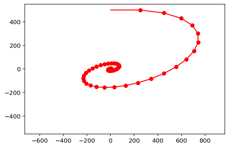
Today we deepen our study of linear dynamical systems,

systems that evolve according to the equation:

\[\mathbf{x}_{k+1} = A\mathbf{x}_k.\]

Let’s look at some examples of how such dynamical systems can evolve in $\mathbb{R}^2$.

First we’ll look at the system corresponding to:

\[\begin{split} A = \begin{bmatrix}\cos 0.1&-\sin 0.1\\\sin 0.1&\cos 1.0\end{bmatrix} \end{split}\]

sl.display_saved_anim('images/L17-ex1.mp4')

Next let’s look at the system corresponding to:

\[\begin{split} A = \begin{bmatrix}1.1&0\\0&0.9\end{bmatrix} \end{split}\]

sl.display_saved_anim('images/L17-ex2.mp4')

Next let’s look at the system corresponding to:

\[\begin{split} A = \begin{bmatrix}0.8&0.5\\-0.1&1.0\end{bmatrix} \end{split}\]

sl.display_saved_anim('images/L17-ex3.mp4')

There are very different things happening in these three cases!

Can we find a general method for understanding what is going on in each case?

The study of eigenvalues and eigenvectors is the key to acquiring that understanding.

We will see that to understand each case, we need to learn how to extract the eigenvalues and eigenvectors of $A$.

Finding $\lambda$¶

In the last lecture we saw that, if we know an eigenvalue $\lambda$ of a matrix $A,$ then computing the corresponding eigenspace can be done by constructing a basis for $\operatorname{Nul}\, (A-\lambda I).$

Today we’ll discuss how to determine the eigenvalues of a matrix $A$.

The theory will make use of the determinant of a matrix.

Let’s recall that the determinant of a $2\times 2$ matrix $A = \begin{bmatrix}a&b\\c&d\end{bmatrix}$ is $ad-bc.$

We also have learned that $A$ is invertible if and only if its determinant is not zero.

(Recall that the inverse of of $A$ is $\frac{1}{ad-bc}\begin{bmatrix}d&-b\\-c&a\end{bmatrix}).$

Let’s use these facts to help us find the eigenvalues of a $2\times 2$ matrix.

Example. Find the eigenvalues of $A = \begin{bmatrix}2&3\\3&-6\end{bmatrix}.$

Solution. We must find all scalars $\lambda$ such that the matrix equation

\[(A-\lambda I)\mathbf{x} = {\bf 0}\]

has a nontrivial solution.

By the Invertible Matrix Theorem, this problem is equivalent to finding all $\lambda$ such that the matrix $A-\lambda I$ is not invertible.

Now,

\[\begin{split} A - \lambda I = \begin{bmatrix}2&3\\3&-6\end{bmatrix} - \begin{bmatrix}\lambda&0\\0&\lambda\end{bmatrix} = \begin{bmatrix}2-\lambda&3\\3&-6-\lambda\end{bmatrix}.\end{split}\]

We know that $A$ is not invertible exactly when its determinant is zero.

So the eigenvalues of $A$ are the solutions of the equation

\[\begin{split}\det(A-\lambda I) = \det\begin{bmatrix}2-\lambda&3\\3&-6-\lambda\end{bmatrix} = 0.\end{split}\]

Since $\det\begin{bmatrix}a&b\\c&d\end{bmatrix} = ad-bc,$ then

\[\det(A-\lambda I) = (2-\lambda)(-6-\lambda)-(3)(3)\]

\[ = -12 + 6\lambda -2\lambda + \lambda^2 - 9\]

\[= \lambda^2+4\lambda-21\]

\[=(\lambda-3)(\lambda + 7)\]

If $\det(A-\lambda I) = 0,$ then $\lambda = 3$ or $\lambda = -7.$ So the eigenvalues of $A$ are $3$ and $-7$.

Question Time! Q17.1

The same idea works for $n\times n$ matrices – but, for that, we need to define a determinant for larger matrices.

Determinants.

Previously, we’ve defined a determinant for a $2\times 2$ matrix.

To find eigenvalues for larger matrices, we need to define the determinant for any sized (ie, $n\times n$) matrix.

Definition. Let $A$ be an $n\times n$ matrix, and let $U$ be any echelon form obtained from $A$ by row replacements and row interchanges (no row scalings), and let $r$ be the number of such row interchanges.

Then the determinant of $A$, written as $\det A$, is $(-1)^r$ times the product of the diagonal entries $u_{11},\dots,u_{nn}$ in $U$.

If $A$ is invertible, then $u_{11},\dots,u_{nn}$ are all pivots.

If $A$ is not invertible, then at least one diagonal entry is zero, and so the product $u_{11} \dots u_{nn}$ is zero.

In other words:

\[\begin{split}\det\ A = \left\{\begin{array}{ll}(-1)^r\cdot\left(\mbox{product of pivots in $U$}\right),&\mbox{when $A$ is invertible}\\ 0,&\mbox{when $A$ is not invertible}\end{array}\right.\end{split}\]

Example. Compute $\det A$ for $A = \begin{bmatrix}1&5&0\\2&4&-1\\0&-2&0\end{bmatrix}.$

Solution. The following row reduction uses one row interchange:

\[\begin{split}A \sim \begin{bmatrix}1&5&0\\0&-6&-1\\0&-2&0\end{bmatrix} \sim \begin{bmatrix}1&5&0\\0&-2&0\\0&-6&-1\end{bmatrix} \sim \begin{bmatrix}1&5&0\\0&-2&0\\0&0&-1\end{bmatrix}.\end{split}\]

So $\det A$ equals $(-1)^1(1)(-2)(-1) = (-2).$

The remarkable thing is that any other way of computing the echelon form gives the same determinant. For example, this row reduction does not use a row interchange:

\[\begin{split}A \sim \begin{bmatrix}1&5&0\\0&-6&-1\\0&-2&0\end{bmatrix} \sim \begin{bmatrix}1&5&0\\0&-6&-1\\0&0&1/3\end{bmatrix}.\end{split}\]

Using this echelon form to compute the determinant yields $(-1)^0(1)(-6)(1/3) = -2,$ the same as before.

Question Time! Q17.2

Invertibility.

The formula for the determinant shows that $A$ is invertible if and only if $\det A$ is nonzero.

We have yet another part to add to the Invertible Matrix Theorem:

Let $A$ be an $n\times n$ matrix. Then $A$ is invertible if and only if:

The number 0 is not an eigenvalue of $A$.
The determinant of $A$ is not zero.

Some facts about determinants (proved in the book):

$\det AB = (\det A) (\det B).$
$\det A^T = \det A.$
If $A$ is triangular, then $\det A$ is the product of the entries on the main diagonal of $A$.

The Characteristic Equation¶

So, $A$ is invertible if and only if $\det A$ is not zero.

To return to the question of how to compute eigenvalues of $A,$ recall that $\lambda$ is an eigenvalue if and only if $(A-\lambda I)$ is not invertible.

We capture this fact using the characteristic equation:

\[\det(A-\lambda I) = 0.\]

We can conclude that $\lambda$ is an eigenvalue of an $n\times n$ matrix $A$ if and only if $\lambda$ satisfies the characteristic equation $\det(A-\lambda I) = 0.$

Example. Find the characteristic equation of

\[\begin{split}A = \begin{bmatrix}5&-2&6&-1\\0&3&-8&0\\0&0&5&4\\0&0&0&1\end{bmatrix}\end{split}\]

Solution. Form $A - \lambda I,$ and note that $\det A$ is the product of the entries on the diagonal of $A,$ if $A$ is triangular.

\[\begin{split}\det(A-\lambda I) = \det\begin{bmatrix}5-\lambda&-2&6&-1\\0&3-\lambda&-8&0\\0&0&5-\lambda&4\\0&0&0&1-\lambda\end{bmatrix}\end{split}\]

\[=(5-\lambda)(3-\lambda)(5-\lambda)(1-\lambda).\]

So the characteristic equation is:

\[(\lambda-5)^2(\lambda-3)(\lambda-1) = 0.\]

Expanding this out we get:

\[\lambda^4 - 14\lambda^3 + 68 \lambda^2 - 130\lambda + 75 = 0.\]

Notice that, once again, $\det(A-\lambda I)$ is a polynomial in $\lambda$.

In fact, for any $n\times n$ matrix, $\det(A-\lambda I)$ is a polynomial of degree $n$, called the characteristic polynomial of $A$.

We say that the eigenvalue 5 in this example has multiplicity 2, because $(\lambda -5)$ occures two times as a factor of the characteristic polynomial. In general, the mutiplicity of an eigenvalue $\lambda$ is its multiplicity as a root of the characteristic equation.

Example. The characteristic polynomial of a $6\times 6$ matrix is $\lambda^6 - 4\lambda^5 - 12\lambda^4.$ Find the eigenvalues and their multiplicity.

Solution Factor the polynomial

\[\lambda^6 - 4\lambda^5 - 12\lambda^4 = \lambda^4(\lambda^2-4\lambda-12) = \lambda^4(\lambda-6)(\lambda+2)\]

So the eigenvalues are 0 (with multiplicity 4), 6, and -2.

Since the characteristic polynomial for an $n\times n$ matrix has degree $n,$ the equation has $n$ roots, counting multiplicities – provided complex numbers are allowed.

Note that even for a real matrix, eigenvalues may sometimes be complex.

Practical Issues.

These facts show that there is, in principle, a way to find eigenvalues of any matrix. However, you need not compute eigenvalues for matrices larger than $2\times 2$ by hand. For any matrix $3\times 3$ or larger, you should use a computer.

Similarity¶

An important concept for things that come later is the notion of similar matrices.

Definition. If $A$ and $B$ are $n\times n$ matrices, then $A$ is similar to $B$ if there is an invertible matrix $P$ such that $P^{-1}AP = B,$ or, equivalently, $A = PBP^{-1}.$

Similarity is symmetric, so if $A$ is similar to $B$, then $B$ is similar to $A$. Hence we just say that $A$ and $B$ are similar.

Changing $A$ into $B$ is called a similarity transformation.

An important way to think of similarity between $A$ and $B$ is that they have the same eigenvalues.

Theorem. If $n\times n$ matrices $A$ and $B$ are similar, then they have the same characteristic polynomial, and hence the same eigenvalues (with the same multiplicities.)

Proof. If $B = P^{-1}AP,$ then

\[B - \lambda I = P^{-1}AP - \lambda P^{-1}P\]

\[ = P^{-1}(AP-\lambda P)\]

\[ = P^{-1}(A-\lambda I)P\]

Now let’s construct the characteristic polynomial by taking the determinant:

\[\det(B-\lambda I) = \det[P^{-1}(A-\lambda I)P]\]

Using the properties of determinants we discussed earlier, we compute:

\[ = \det(P^{-1})\cdot\det(A-\lambda I)\cdot\det(P).\]

Since $\det(P^{-1})\cdot\det(P) = \det(P^{-1}P) = \det I = 1,$ we can see that

\[\det(B-\lambda I) = \det(A - \lambda I).\]

Markov Chains¶

Let’s return to the problem of solving a Markov Chain.

At this point, we can place the theory of Markov Chains into the broader context of eigenvalues and eigenvectors.

Theorem. The largest eigenvalue of a Markov Chain is 1.

Proof. First of all, it is obvious that 1 is an eigenvalue of a Markov chain since we know that every Markov Chain $A$ has a steady-state vector $\mathbf{v}$ such that $A\mathbf{v} = \mathbf{v}.$

To prove that 1 is the largest eigenvalue, recall that each column of a Markov Chain sums to 1.

Then, consider the sum of the values in the vector $A\mathbf{x}$.

\[\begin{split}A\mathbf{x} = \begin{bmatrix}a_{11}&\dots &a_{1n}\\\vdots&\ddots&\vdots\\a_{n1}&\dots&a_{nn}\end{bmatrix}\begin{bmatrix}x_1\\\vdots\\x_n\end{bmatrix} = \begin{bmatrix}a_{11}x_1 + \dots + a_{1n}x_n\\\vdots\\ a_{n1}x_1 + \dots + a_{nn}x_n\end{bmatrix}.\end{split}\]

Let’s just sum the first terms in each component of $A\mathbf{x}$:

\[ a_{11}x_1 + a_{21}x_1 + \dots + a_{n1}x_1 = x_1 \sum_i a_{i1} = x_1. \]

So we can see that the sum of all terms in $A\mathbf{x}$ is equal to $x_1 + x_2 + \dots + x_n$ – i.e., the sum of all terms in $\mathbf{x}$.

So there can be no $\lambda > 1$ such that $A\mathbf{x} = \lambda \mathbf{x}.$

A complete solution for the evolution of a Markov Chain.

Previously, we were only able to ask about the “eventual” steady state of a Markov Chain.

But a crucial question is: how long does it take for a particular Markov Chain to reach steady state from some initial starting condition?

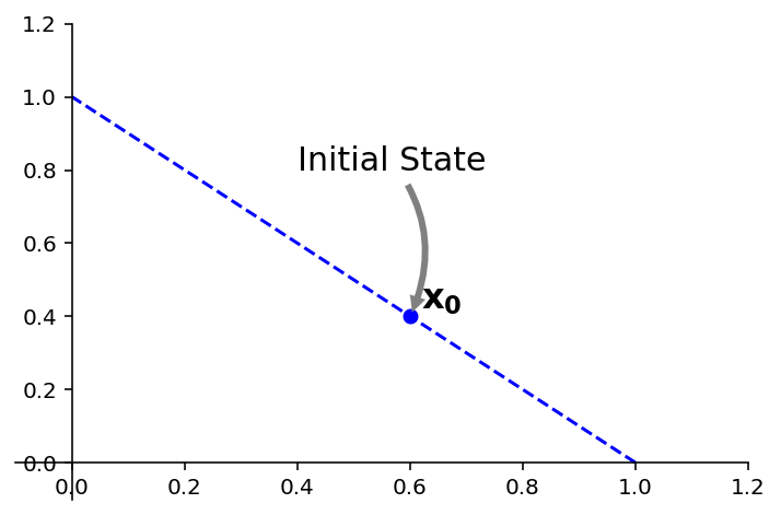
Let’s use an example: we previously studied the Markov Chain defined by $A = \begin{bmatrix}0.95&0.03\\0.05&0.97\end{bmatrix}.$

Let’s ask how long until it reaches steady state, from the starting point defined as $\mathbf{x}_0 = \begin{bmatrix}0.6\\0.4\end{bmatrix}.$

Remember that $x_0$ is probability vector – its entries are nonnegative and sum to 1.

ax = ut.plotSetup(-0.1,1.2,-0.1,1.2)
ut.centerAxes(ax)
A = np.array([[0.95,0.03],[0.05,0.97]])
v1 = np.array([0.375,0.625])
v2 = np.array([0.225,-0.225])
x0 = v1 + v2
#
ax.plot([1,0],[0,1],'b--')
ax.plot(x0[0],x0[1],'bo')
ax.text(x0[0]+0.02,x0[1]+0.02,r'${\bf x_0}$',size=16)
#ax.text(A.dot(x0)[0]+0.2,A.dot(x0)[1]+0.2,r'$A{\bf x_0}$',size=16)
# ax.plot([-10,10],[5*10/6.0,-5*10/6.0],'b-')
#
ax.annotate('Initial State', xy=(x0[0], x0[1]),  xycoords='data',
                xytext=(0.4, 0.8), textcoords='data',
                size=15,
                #bbox=dict(boxstyle="round", fc="0.8"),
                arrowprops={'arrowstyle': 'simple',
                                'fc': '0.5', 
                                'ec': 'none',
                                'connectionstyle' : 'arc3,rad=-0.3'},
                );

Using the methods we studied today, we can find the characteristic equation:

\[\lambda^2 -1.92\lambda +0.92 \]

Using the quadratic formula, we find the roots of this equation to be 1 and 0.92. (Note that, as expected, 1 is the largest eigenvalue.)

Next, using the methods in the previous lecture, we find a basis for each eigenspace of $A$ (each nullspace of $A-\lambda I$).

For $\lambda = 1$, a corresponding eigenvector is $\mathbf{v}_1 = \begin{bmatrix}3\\5\end{bmatrix}.$

For $\lambda = 0.92$, a corresponding eigenvector is $\mathbf{v}_2 = \begin{bmatrix}1\\-1\end{bmatrix}.$

Next, we write $\mathbf{x}_0$ as a linear combination of $\mathbf{v}_1$ and $\mathbf{v}_2.$ This can be done because $\{\mathbf{v}_1,\mathbf{v}_2\}$ is obviously a basis for $\mathbb{R}^2.$

To write $\mathbf{x}_0$ this way, we want to solve the vector equation

\[c_1\mathbf{v}_1 + c_2\mathbf{v}_2 = \mathbf{x}_0\]

In other words:

\[\begin{split}[\mathbf{v}_1\;\mathbf{v}_2]\begin{bmatrix}c_1\\c_2\end{bmatrix} = \mathbf{x}_0.\end{split}\]

The matrix $[\mathbf{v}_1\;\mathbf{v}_2]$ is invertible, so,

\[\begin{split}\begin{bmatrix}c_1\\c_2\end{bmatrix} = [\mathbf{v}_1\;\mathbf{v}_2]^{-1} \mathbf{x}_0 = \begin{bmatrix}3&1\\5&-1\end{bmatrix}^{-1}\begin{bmatrix}0.6\\0.4\end{bmatrix}.\end{split}\]

\[\begin{split} = \frac{1}{-8}\begin{bmatrix}-1&-1\\-5&3\end{bmatrix}\begin{bmatrix}0.6\\0.4\end{bmatrix} = \begin{bmatrix}0.125\\0.225\end{bmatrix}.\end{split}\]

So, now we can put it all together.

We know that

\[\mathbf{x}_0 = c_1\mathbf{v}_1 + c_2\mathbf{v}_2\]

and we know the values of $c_1, c_2$ that make this true.

So let’s compute each $\mathbf{x}_k$:

\[\mathbf{x}_1 = A\mathbf{x}_0 = c_1A\mathbf{v}_1 + c_2A\mathbf{v}_2\]

\[ = c_1\mathbf{v}_1 + c_2(0.92)\mathbf{v}_2.\]

Now note the power of the eigenvalue approach:

\[\mathbf{x}_2 = A\mathbf{x}_1 = c_1A\mathbf{v}_1 + c_2(0.92)A\mathbf{v}_2\]

\[=c_1\mathbf{v}_2 + c_2(0.92)^2\mathbf{v}_2.\]

And so in general: $$\mathbf{x}_k = c_1\mathbf{v}_1 + c_2(0.92)^k\mathbf{v}_2\;\;\;(k = 0, 1, 2, \dots)$$

And using the $c_1$ and $c_2$ and $\mathbf{v}_1,$ $\mathbf{v}_2$ we computed above:

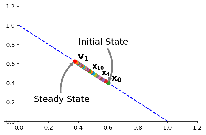
\[\begin{split}\mathbf{x}_k = 0.125\begin{bmatrix}3\\5\end{bmatrix} + 0.225(0.92)^k\begin{bmatrix}1\\-1\end{bmatrix}\;\;\;(k = 0, 1, 2, \dots)\end{split}\]

This explicit formula for $\mathbf{x}_k$ gives the solution of the Markov Chain $\mathbf{x}_{k+1} = A\mathbf{x}_k$ starting from the initial state $\mathbf{x}_0$.

In other words: $$\mathbf{x}_0 = 0.125\begin{bmatrix}3\\5\end{bmatrix} + 0.225\begin{bmatrix}1\\-1\end{bmatrix}$$\mathbf{x}_1 = 0.125\begin{bmatrix}3\\5\end{bmatrix} + 0.207\begin{bmatrix}1\\-1\end{bmatrix}$$\mathbf{x}_2 = 0.125\begin{bmatrix}3\\5\end{bmatrix} + 0.190\begin{bmatrix}1\\-1\end{bmatrix}$$\mathbf{x}_3 = 0.125\begin{bmatrix}3\\5\end{bmatrix} + 0.175\begin{bmatrix}1\\-1\end{bmatrix}$$ ... $$\mathbf{x}_\infty = 0.125\begin{bmatrix}3\\5\end{bmatrix}$$

As $k\rightarrow\infty$, $(0.92)^k\rightarrow0$.

Thus $\mathbf{x}_k \rightarrow 0.125\mathbf{v}_1 = \begin{bmatrix}0.375\\0.625\end{bmatrix}.$

ax = ut.plotSetup(-0.1,1.2,-0.1,1.2)
ut.centerAxes(ax)
A = np.array([[0.95,0.03],[0.05,0.97]])
v1 = np.array([0.375,0.625])
v2 = np.array([0.225,-0.225])
x0 = v1 + v2
#
ax.plot([1,0],[0,1],'b--')
ax.text(v1[0]+0.02,v1[1]+0.02,r'${\bf v_1}$',size=16)
ax.plot(x0[0],x0[1],'bo')
v = np.zeros((40,2))
for i in range(40):
    v[i] = v1+(0.92**i)*v2
    ax.plot(v[i,0],v[i,1],'o')
ax.text(v[4][0]+0.02,v[4][1]+0.02,r'${\bf x_4}$',size=12)
ax.text(v[10][0]+0.02,v[10][1]+0.02,r'${\bf x_{10}}$',size=12)
ax.text(x0[0]+0.02,x0[1]+0.02,r'${\bf x_0}$',size=16)
ax.plot(v1[0],v1[1],'ro')
#ax.text(A.dot(x0)[0]+0.2,A.dot(x0)[1]+0.2,r'$A{\bf x_0}$',size=16)
# ax.plot([-10,10],[5*10/6.0,-5*10/6.0],'b-')
#
ax.annotate('Steady State', xy=(v1[0], v1[1]),  xycoords='data',
                xytext=(0.1, 0.2), textcoords='data',
                size=15,
                #bbox=dict(boxstyle="round", fc="0.8"),
                arrowprops={'arrowstyle': 'simple',
                                'fc': '0.5', 
                                'ec': 'none',
                                'connectionstyle' : 'arc3,rad=-0.3'},
                )
ax.annotate('Initial State', xy=(v[0,0], v[0,1]),  xycoords='data',
                xytext=(0.4, 0.8), textcoords='data',
                size=15,
                #bbox=dict(boxstyle="round", fc="0.8"),
                arrowprops={'arrowstyle': 'simple',
                                'fc': '0.5', 
                                'ec': 'none',
                                'connectionstyle' : 'arc3,rad=-0.3'},
                )
print('')

Linear Algebra, Geometry, and Computation

The Characteristic Equation¶

Finding \(\lambda\)¶

The Characteristic Equation¶

Similarity¶

Markov Chains¶