# for QR codes use inline
# %matplotlib inline
# qr_setting = 'url'
# qrviz_setting = 'show'
#
# for lecture use notebook
%matplotlib inline
qr_setting = None
#
%config InlineBackend.figure_format='retina'
# import libraries
import numpy as np
import matplotlib as mp
import pandas as pd
import matplotlib.pyplot as plt
import laUtilities as ut
import slideUtilities as sl
import demoUtilities as dm
import pandas as pd
from importlib import reload
from datetime import datetime
from IPython.display import Image
from IPython.display import display_html
from IPython.display import display
from IPython.display import Math
from IPython.display import Latex
from IPython.display import HTML;
Orthogonal Sets and Projection
# image from NYT - https://www.nytimes.com/store/me-38-my-human-2004-nsap364p.html
display(Image("images/skaters.jpg", width=350))
Today we deepen our study of geometry.
In the last lecture we focused on points, lines, and angles.
Today we take on more challenging geometric notions that bring in sets of vectors and subspaces.
Within this realm, we will focus on orthogonality and a new notion called projection.
First of all, today we’ll study the properties of sets of orthogonal vectors.
These can be very useful.
Orthogonal Sets
A set of vectors \(\{\mathbf{u}_1,\dots,\mathbf{u}_p\}\) in \(\mathbb{R}^n\) is said to be an orthogonal set if each pair of distinct vectors from the set is orthogonal, i.e.,
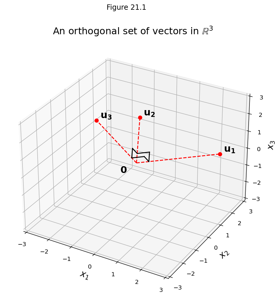
Example. Show that \(\{\mathbf{u}_1,\mathbf{u}_2,\mathbf{u}_3\}\) is an orthogonal set, where
Solution. Consider the three possible pairs of distinct vectors, namely, \(\{\mathbf{u}_1,\mathbf{u}_2\}, \{\mathbf{u}_1,\mathbf{u}_3\},\) and \(\{\mathbf{u}_2,\mathbf{u}_3\}.\)
Each pair of distinct vectors is orthogonal, and so \(\{\mathbf{u}_1,\mathbf{u}_2, \mathbf{u}_3\}\) is an orthogonal set.
In three-space they describe three lines that we say are mutually perpendicular.
fig = ut.three_d_figure((21, 1), fig_desc = 'An orthogonal set of vectors',
                        xmin = -3, xmax = 3, ymin = -3, ymax = 3, zmin = -3, zmax = 3,
                        figsize = (12, 8), qr = qr_setting)
u1 = np.array([3, 1, 1])
u2 = np.array([-1, 2, 1])
u3 = np.array([-1/2, -2, 7/2])
origin = np.array([0, 0, 0])
fig.plotLine([origin, u1], 'r', '--')
fig.plotPoint(u1[0], u1[1], u1[2], 'r')
fig.text(u1[0]+.1, u1[1]+.1, u1[2]+.1, r'$\bf u_1$', 'u1', size=16, color='k')
fig.plotLine([origin, u2], 'r', '--')
fig.plotPoint(u2[0], u2[1], u2[2], 'r')
fig.text(u2[0]+.1, u2[1]+.1, u2[2]+.1, r'$\bf u_2$', 'u2', size=16, color='k')
fig.plotLine([origin, u3], 'r', '--')
fig.plotPoint(u3[0], u3[1], u3[2], 'r')
fig.text(u3[0]+.1, u3[1]+.1, u3[2]+.1, r'$\bf u_3$', 'u3', size=16, color = 'k')
fig.text(origin[0]-.45, origin[1]-.45, origin[2]-.45, r'$\bf 0$', 0, size = 16)
fig.plotPerpSym(origin, u1, u2, 0.5)
fig.plotPerpSym(origin, u3, u2, 0.5)
fig.plotPerpSym(origin, u3, u1, 0.5)
fig.set_title(r'An orthogonal set of vectors in $\mathbb{R}^3$', 'An orthogonal set of vectors in R3', size = 16)
fig.save();
Question Time! Q21.1
Orthogonal Sets Must be Independent
Orthogonal sets are very nice to work with. First of all, we will show that any orthogonal set must be linearly independent.
Theorem. If \(S = \{\mathbf{u}_1,\dots,\mathbf{u}_p\}\) is an orthogonal set of nonzero vectors in \(\mathbb{R}^n,\) then \(S\) is linearly independent.
Proof. We will prove that there is no linear combination of the vectors in \(S\) with nonzero coefficients that yields the zero vector.
Our proof strategy will be:
we will show that for any linear combination of the vectors in \(S\):
if the combination is the zero vector,
then all coefficients of the combination must be zero.
Specifically:
Assume \({\bf 0} = c_1\mathbf{u}_1 + \dots + c_p\mathbf{u}_p\) for some scalars \(c_1,\dots,c_p\). Then:
Because \(\mathbf{u}_1\) is orthogonal to \(\mathbf{u}_2,\dots,\mathbf{u}_p\):
Since \(\mathbf{u}_1\) is nonzero, \(\mathbf{u}_1^T\mathbf{u}_1\) is not zero and so \(c_1 = 0\).
We can use the same kind of reasoning to show that, \(c_2,\dots,c_p\) must be zero.
In other words, there is no nonzero combination of \(\mathbf{u}_i\)’s that yields the zero vector …
… so \(S\) is linearly independent.
Notice that since \(S\) is a linearly independent set, it is a basis for the subspace spanned by \(S\).
This leads us to a new kind of basis.
Orthogonal Basis
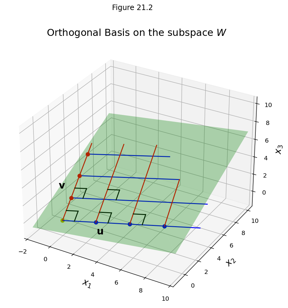
Definition. An orthogonal basis for a subspace \(W\) of \(\mathbb{R}^n\) is a basis for \(W\) that is also an orthogonal set.
For example, consider
Note that \(\mathbf{u}^T\mathbf{v} = 0.\) Hence they form an orthogonal basis for their span.
Here is the subspace \(W = \mbox{Span}\{\mathbf{u},\mathbf{v}\}\):
fig = ut.three_d_figure((21, 2), fig_desc = 'Orthogonal Basis on the subspace W', figsize = (8, 8),
                        xmin = -2, xmax = 10, ymin = -1, ymax = 10, zmin = -1, zmax = 10, qr = qr_setting)

v = 1/2 * np.array([-1, 4, 2])
u = 1/3 * np.array([8, 1, 2])
vpos = v + 0.4 * v - 0.5 * u
upos = u - 0.5 * v + 0.15 * u
fig.text(vpos[0], vpos[1], vpos[2], r'$\bf v$', 'v', size=16)
fig.text(upos[0], upos[1], upos[2], r'$\bf u$', 'u', size=16)
# fig.text(3*u[0]+2*v[0], 3*u[1]+2*v[1], 3*u[2]+2*v[2]+1, r'$\bf 2v_1+3v_2$', '2 v1 + 3 v2', size=16)
# plotting the span of v
fig.plotSpan(u, v, 'Green')
# blue grid lines
fig.plotPoint(0, 0, 0, 'y')
fig.plotPoint(u[0], u[1], u[2], 'b')
fig.plotPoint(2*u[0], 2*u[1], 2*u[2],'b')
fig.plotPoint(3*u[0], 3*u[1], 3*u[2], 'b')
fig.plotLine([[0, 0, 0], 4*u], color='b')
fig.plotLine([v, v+4*u], color='b')
fig.plotLine([2*v, 2*v+3*u], color='b')
fig.plotLine([3*v, 3*v+2.5*u], color='b')
# red grid lines
fig.plotPoint(v[0], v[1], v[2], 'r')
fig.plotPoint(2*v[0], 2*v[1], 2*v[2], 'r')
fig.plotPoint(3*v[0], 3*v[1], 3*v[2], 'r')
fig.plotLine([[0, 0, 0], 3.5*v], color='r')
fig.plotLine([u, u+3.5*v], color='r')
fig.plotLine([2*u, 2*u+3.5*v], color='r')
fig.plotLine([3*u, 3*u+2*v], color='r')
#
# fig.plotPoint(3*u[0]+2*v[0], 3*u[1]+2*v[1], 3*u[2]+2*v[2], color='m')
# plotting the axes
#fig.plotIntersection([0,0,1,0], [0,1,0,0], color='Black')
#fig.plotIntersection([0,0,1,0], [1,0,0,0], color='Black')
#fig.plotIntersection([0,1,0,0], [1,0,0,0], color='Black')
#
fig.plotPerpSym(np.array([0, 0, 0]), v, u, 1)
fig.plotPerpSym(u, v+u, u+u, 1)
fig.plotPerpSym(2*u, v+2*u, 3*u, 1)
#
fig.plotPerpSym(np.array([0, 0, 0])+v, 2*v, v+u, 1)
fig.plotPerpSym(u+v, 2*v+u, v+2*u, 1)
#
fig.set_title(r'Orthogonal Basis on the subspace $W$', 'Orthogonal Basis on the subspace W', size=16)
fig.save()
We have seen that for any subspace, there may be many different sets of vectors that can serve as a basis for \(W\).
For example, let’s say we have a basis \(\mathcal{B} = \{\mathbf{u}_1, \mathbf{u}_2, \mathbf{u}_3\}.\)
We know that to compute the coordinates of \(\mathbf{y}\) in this basis, we need to solve the linear system:
or
In general, we’d need to perform Gaussian Elimination, or matrix inversion, or some other complex method to do this.
However an orthogonal basis is a particularly nice basis, because the weights (coordinates) of any point can be computed easily and simply.
Let’s see how:
Theorem. Let \(\{\mathbf{u}_1,\dots,\mathbf{u}_p\}\) be an orthogonal basis for a subspace \(W\) of \(\mathbb{R}^n\). For each \(\mathbf{y}\) in \(W,\) the weights of the linear combination
are given by
Proof.
Let’s consider the inner product of \(\mathbf{y}\) and one of the \(\mathbf{u}\) vectors — say, \(\mathbf{u}_1\).
As we saw in the last proof, the orthogonality of \(\{\mathbf{u}_1,\dots,\mathbf{u}_p\}\) means that
Since \(\mathbf{u}_1^T\mathbf{u}_1\) is not zero (why?), the equation above can be solved for \(c_1.\)
Thus:
To find any other \(c_j,\) compute \(\mathbf{y}^T\mathbf{u}_j\) and solve for \(c_j\).
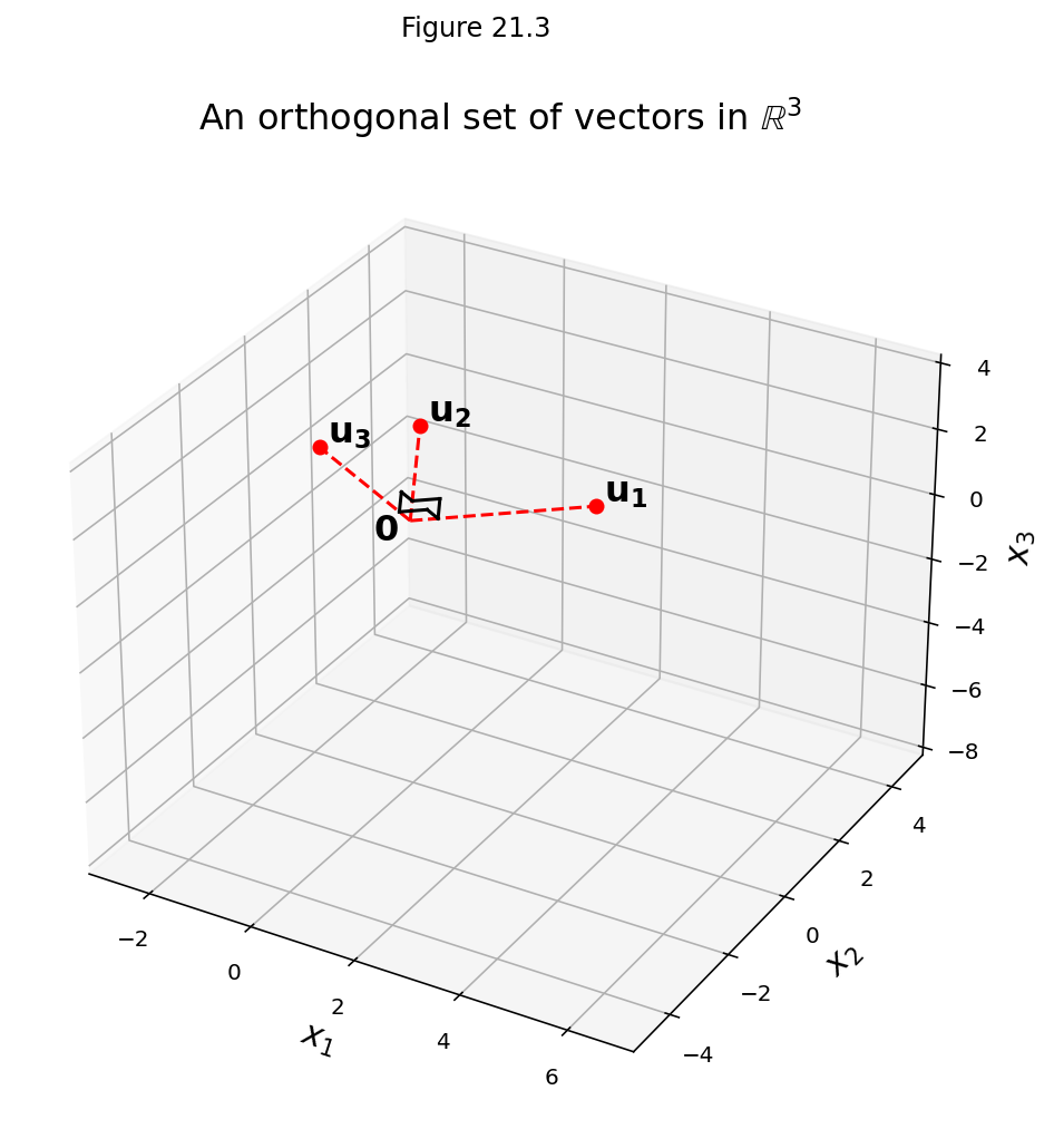
Example. The set \(S\) which we saw earlier, ie,
is an orthogonal basis for \(\mathbb{R}^3.\)
import importlib
importlib.reload(ut)
fig = ut.three_d_figure((21, 3), fig_desc = 'An orthogonal set of vectors',
                        xmin = -3, xmax = 7, ymin = -5, ymax = 5, zmin = -8, zmax = 4,
                        figsize = (12, 8), qr = qr_setting, equalAxes = False)
u1 = np.array([3, 1, 1])
u2 = np.array([-1, 2, 1])
u3 = np.array([-1/2, -2, 7/2])
origin = np.array([0, 0, 0])
fig.plotLine([origin, u1], 'r', '--')
fig.plotPoint(u1[0], u1[1], u1[2], 'r')
fig.text(u1[0]+.1, u1[1]+.1, u1[2]+.1, r'$\bf u_1$', 'u1', size=16, color='k')
fig.plotLine([origin, u2], 'r', '--')
fig.plotPoint(u2[0], u2[1], u2[2], 'r')
fig.text(u2[0]+.1, u2[1]+.1, u2[2]+.1, r'$\bf u_2$', 'u2', size=16, color='k')
fig.plotLine([origin, u3], 'r', '--')
fig.plotPoint(u3[0], u3[1], u3[2], 'r')
fig.text(u3[0]+.1, u3[1]+.1, u3[2]+.1, r'$\bf u_3$', 'u3', size=16, color = 'k')
fig.text(origin[0]-.45, origin[1]-.45, origin[2]-.45, r'$\bf 0$', 0, size = 16)
fig.plotPerpSym(origin, u1, u2, 0.5)
fig.plotPerpSym(origin, u3, u2, 0.5)
fig.plotPerpSym(origin, u3, u1, 0.5)
fig.set_title(r'An orthogonal set of vectors in $\mathbb{R}^3$', 'An orthogonal set of vectors in R3', size = 16)
fig.save();
Then, express the vector \(\mathbf{y} = \begin{bmatrix}6\\1\\-8\end{bmatrix}\) as a linear combination of the vectors in \(S\).
That is, find \(\mathbf{y}\)’s coordinates in the basis \(S\) — i.e., in the coordinate system \(S\).
Solution. Compute
So
fig = ut.three_d_figure((21, 4), fig_desc = 'y in an orthogonal basis',
                        xmin = -3, xmax = 7, ymin = -5, ymax = 5, zmin = -8, zmax = 4,
                        figsize = (12, 8), qr = qr_setting, equalAxes = False)
u1 = np.array([3, 1, 1])
u2 = np.array([-1, 2, 1])
u3 = np.array([-1/2, -2, 7/2])
origin = np.array([0, 0, 0])
#
fig.plotLine([origin, u1], 'r', '--')
fig.plotPoint(u1[0], u1[1], u1[2], 'r')
fig.text(u1[0]+.1, u1[1]+.1, u1[2]+.1, r'$\bf u_1$', 'u1', size=16, color='k')
#
fig.plotLine([origin, u2], 'r', '--')
fig.plotPoint(u2[0], u2[1], u2[2], 'r')
fig.text(u2[0]+.1, u2[1]+.1, u2[2]+.1, r'$\bf u_2$', 'u2', size=16, color='k')
#
fig.plotLine([origin, u3], 'r', '--')
fig.plotPoint(u3[0], u3[1], u3[2], 'r')
fig.text(u3[0]+.1, u3[1]+.1, u3[2]+.1, r'$\bf u_3$', 'u3', size=16, color = 'k')
#
fig.text(origin[0]-.45, origin[1]-.45, origin[2]-.45, r'$\bf 0$', 0, size = 16)
#
fig.plotPerpSym(origin, u1, u2, 0.5)
fig.plotPerpSym(origin, u3, u2, 0.5)
fig.plotPerpSym(origin, u3, u1, 0.5)
#
y = u1 - 2 * u2 - 2 * u3
# print(y)
fig.plotPoint(y[0], y[1], y[2], 'b')
fig.text(y[0]-2, y[1]+.1, y[2]+.1, r'$\bf y$ = (6, 1, -8)', 'y = (6, 1, -8)', size=16, color = 'b')
fig.text(y[0]-2, y[1]+.1, y[2]-2.5, r'${\bf y} = 1{\bf u}_1 -2 {\bf u}_2 -2 {\bf u}_3$', 'y = (6, 1, -8)', size=16, color = 'b')
#
fig.set_title(r'${\bf y}$ in an Orthogonal Basis', 'y in an Orthogonal Basis', size = 16)
fig.save();
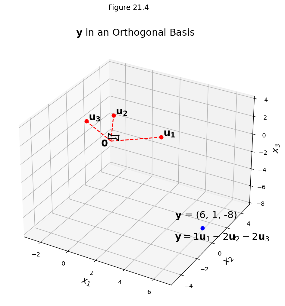
Note how much simpler it is finding the coordinates of \(\mathbf{y}\) in the orthogonal basis,
because each coefficient \(c_1\) can be found separately without matrix operations.
Orthogonal Projection
Now let’s turn to the notion of projection.
In general, a projection happens when we decompose a vector into the sum of other vectors.
Here is the central idea. We will use this a lot over the next couple lectures.
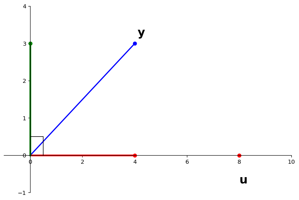
Given a nonzero vector \(\mathbf{u}\) in \(\mathbb{R}^n,\) consider the problem of decomposing a vector \(\mathbf{y}\) in \(\mathbb{R}^n\) into the sum of two vectors:
one that is a multiple of \(\mathbf{u}\), and
one that is orthogonal to \(\mathbf{u}.\)
ax = ut.plotSetup(-1,10,-1,4,(9,6))
ut.centerAxes(ax)
pt = [4., 3.]
plt.plot([0,pt[0]],[0,pt[1]],'b-',lw=2)
plt.plot([0,pt[0]],[0,0],'r-',lw=3)
plt.plot([0,0],[0,pt[1]],'g-',lw=3)
ut.plotVec(ax,pt,'b')
u = np.array([pt[0],0])
v = [0,pt[1]]
ut.plotVec(ax,u)
ut.plotVec(ax,2*u)
ut.plotVec(ax,v,'g')
perpline1, perpline2 = ut.perp_sym(np.array([0,0]), u, v, 0.5)
plt.plot(perpline1[0], perpline1[1], 'k', lw = 1)
plt.plot(perpline2[0], perpline2[1], 'k', lw = 1)
ax.text(2*pt[0],-0.75,r'$\mathbf{u}$',size=20)
ax.text(pt[0]+0.1,pt[1]+0.2,r'$\mathbf{y}$',size=20);
In other words, we wish to write:
where \(\hat{\mathbf{y}} = \alpha\mathbf{u}\) for some scalar \(\alpha\) and \(\mathbf{z}\) is some vector orthogonal to \(\mathbf{u}.\)
ax = ut.plotSetup(-1,10,-1,4,(9,6))
ut.centerAxes(ax)
pt = [4., 3.]
plt.plot([0,pt[0]],[0,pt[1]],'b-',lw=2)
plt.plot([pt[0],pt[0]],[0,pt[1]],'b--',lw=2)
plt.plot([0,pt[0]],[0,0],'r-',lw=3)
plt.plot([0,0],[0,pt[1]],'g-',lw=3)
ut.plotVec(ax,pt,'b')
u = np.array([pt[0],0])
v = [0,pt[1]]
ut.plotVec(ax,u)
ut.plotVec(ax,2*u)
ut.plotVec(ax,v,'g')
ax.text(pt[0],-0.75,r'${\bf \hat{y}}=\alpha{\bf u}$',size=20)
ax.text(2*pt[0],-0.75,r'$\mathbf{u}$',size=20)
ax.text(pt[0]+0.1,pt[1]+0.2,r'$\mathbf{y}$',size=20)
perpline1, perpline2 = ut.perp_sym(np.array([0,0]), u, v, 0.5)
plt.plot(perpline1[0], perpline1[1], 'k', lw = 1)
plt.plot(perpline2[0], perpline2[1], 'k', lw = 1);
# ax.text(0+0.1,pt[1]+0.2,r'$\mathbf{z = y -\hat{y}}$',size=20);
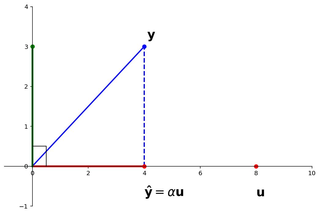
That is, we are given \(\mathbf{y}\) and \(\mathbf{u}\), and asked to compute \(\mathbf{z}\) and \(\hat{\mathbf{y}}.\)
To solve this, assume that we have some \(\alpha\), and with it we compute \(\mathbf{y} - \alpha\mathbf{u} = \mathbf{y}-\hat{\mathbf{y}} = \mathbf{z}.\)
We want \(\mathbf{z}\) to be orthogonal to \(\mathbf{u}.\)
Now \(\mathbf{z} = \mathbf{y} - \alpha{\mathbf{u}}\) is orthogonal to \(\mathbf{u}\) if and only if
That is, the solution in which \(\mathbf{z}\) is orthogonal to \(\mathbf{u}\) happens if and only if
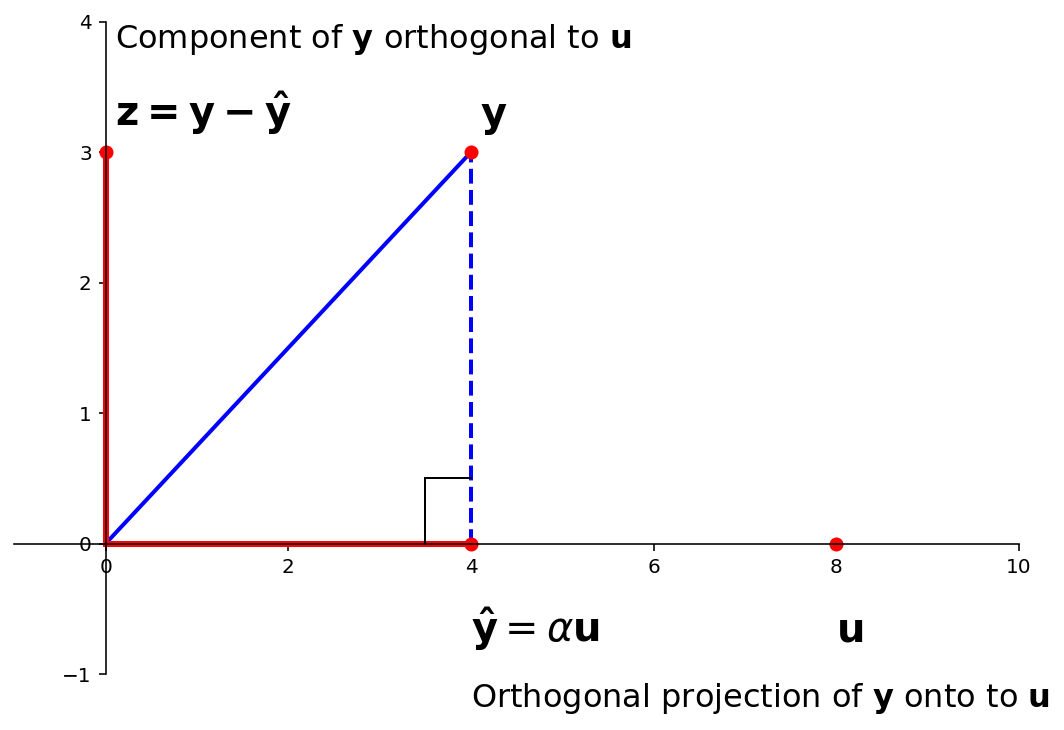
and since \(\hat{\mathbf{y}} = \alpha\mathbf{u}\),
The vector \(\hat{\mathbf{y}}\) is called the orthogonal projection of \(\mathbf{y}\) onto \(\mathbf{u}\), and the vector \(\mathbf{z}\) is called the component of \(\mathbf{y}\) orthogonal to \(\mathbf{u}.\)
sl.hide_code_in_slideshow()
ax = ut.plotSetup(-1,10,-1,4,(9,6))
ut.centerAxes(ax)
pt = [4., 3.]
plt.plot([0,pt[0]],[0,pt[1]],'b-',lw=2)
plt.plot([pt[0],pt[0]],[0,pt[1]],'b--',lw=2)
plt.plot([0,pt[0]],[0,0],'r-',lw=3)
plt.plot([0,0],[0,pt[1]],'r-',lw=3)
ut.plotVec(ax,pt)
u = np.array([pt[0],0])
v = [0,pt[1]]
ut.plotVec(ax,u)
ut.plotVec(ax,2*u)
ut.plotVec(ax,v)
perpline1, perpline2 = ut.perp_sym(np.array([pt[0], 0]), np.array([0,0]), pt, 0.5)
plt.plot(perpline1[0], perpline1[1], 'k', lw = 1)
plt.plot(perpline2[0], perpline2[1], 'k', lw = 1)
ax.text(pt[0],-0.75,r'${\bf \hat{y}}=\alpha{\bf u}$',size=20)
ax.text(2*pt[0],-0.75,r'$\mathbf{u}$',size=20)
ax.text(pt[0]+0.1,pt[1]+0.2,r'$\mathbf{y}$',size=20)
ax.text(0+0.1,pt[1]+0.2,r'$\mathbf{z = y -\hat{y}}$',size=20)
ax.text(0+0.1,pt[1]+0.8,r'Component of $\mathbf{y}$ orthogonal to $\mathbf{u}$',size=16)
ax.text(pt[0],-1.25,r'Orthogonal projection of $\mathbf{y}$ onto to $\mathbf{u}$',size=16);
Projections are onto Subspaces
sl.hide_code_in_slideshow()
ax = ut.plotSetup(-1,10,-1,4,(9,6))
ut.centerAxes(ax)
pt = [4., 3.]
plt.plot([0,pt[0]],[0,pt[1]],'b-',lw=2)
plt.plot([pt[0],pt[0]],[0,pt[1]],'b--',lw=2)
plt.plot([0,pt[0]],[0,0],'r-',lw=3)
plt.plot([0,0],[0,pt[1]],'r-',lw=3)
ut.plotVec(ax,pt)
u = np.array([pt[0],0])
v = [0,pt[1]]
ut.plotVec(ax,u)
ut.plotVec(ax,2*u)
ut.plotVec(ax,v)
perpline1, perpline2 = ut.perp_sym(np.array([pt[0], 0]), np.array([0,0]), pt, 0.5)
plt.plot(perpline1[0], perpline1[1], 'k', lw = 1)
plt.plot(perpline2[0], perpline2[1], 'k', lw = 1)
ax.text(pt[0],-0.75,r'${\bf \hat{y}}=\alpha{\bf u}$',size=20)
ax.text(2*pt[0],-0.75,r'$\mathbf{u}$',size=20)
ax.text(pt[0]+0.1,pt[1]+0.2,r'$\mathbf{y}$',size=20)
ax.text(0+0.1,pt[1]+0.2,r'$\mathbf{z = y -\hat{y}}$',size=20)
ax.text(0+0.1,pt[1]+0.8,r'Component of $\mathbf{y}$ orthogonal to $\mathbf{u}$',size=16)
ax.text(pt[0],-1.25,r'Orthogonal projection of $\mathbf{y}$ onto to $\mathbf{u}$',size=16);

Now, note that if we had scaled \(\mathbf{u}\) by any amount (ie, moved it to the right or the left), we would not have changed the location of \(\hat{\mathbf{y}}.\)
This can be seen as well by replacing \(\mathbf{u}\) with \(c\mathbf{u}\) and recomputing \(\hat{\mathbf{y}}\):
Thus, the projection of \(\mathbf{y}\) is determined by the subspace \(L\) that is spanned by \(\mathbf{u}\) – in other words, the line through \(\mathbf{u}\) and the origin.
Hence sometimes \(\hat{\mathbf{y}}\) is denoted by \(\mbox{proj}_L \mathbf{y}\) and is called the orthogonal projection of \(\mathbf{y}\) onto \(L\).
Specifically:
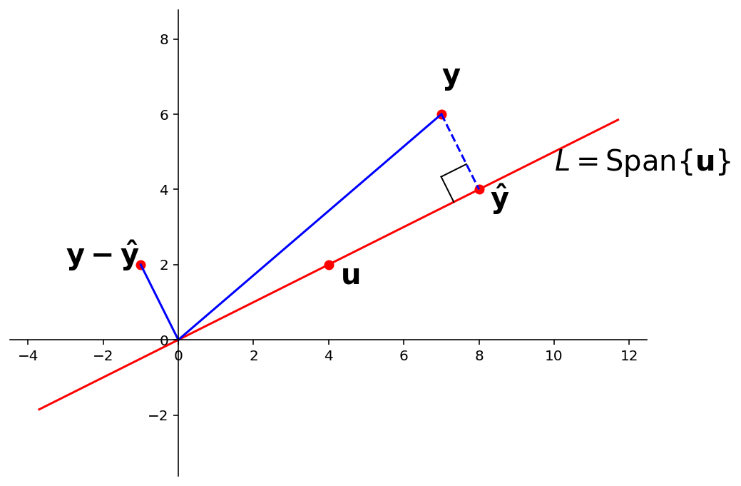
Example. Let \(\mathbf{y} = \begin{bmatrix}7\\6\end{bmatrix}\) and \(\mathbf{u} = \begin{bmatrix}4\\2\end{bmatrix}.\)
Find the orthogonal projection of \(\mathbf{y}\) onto \(\mathbf{u}.\) Then write \(\mathbf{y}\) as the sum of two orthogonal vectors, one in Span\(\{\mathbf{u}\}\), and one orthogonal to \(\mathbf{u}.\)
Solution. Compute
The orthogonal projection of \(\mathbf{y}\) onto \(\mathbf{u}\) is
And the component of \(\mathbf{y}\) orthogonal to \(\mathbf{u}\) is
So
ax = ut.plotSetup(-3,11,-1,7,(8,6))
ut.centerAxes(ax)
plt.axis('equal')
u = np.array([4.,2])
y = np.array([7.,6])
yhat = (y.T.dot(u)/u.T.dot(u))*u
z = y-yhat
ut.plotLinEqn(1.,-2.,0.)
ut.plotVec(ax,u)
ut.plotVec(ax,z)
ut.plotVec(ax,y)
ut.plotVec(ax,yhat)
ax.text(u[0]+0.3,u[1]-0.5,r'$\mathbf{u}$',size=20)
ax.text(yhat[0]+0.3,yhat[1]-0.5,r'$\mathbf{\hat{y}}$',size=20)
ax.text(y[0],y[1]+0.8,r'$\mathbf{y}$',size=20)
ax.text(z[0]-2,z[1],r'$\mathbf{y - \hat{y}}$',size=20)
ax.text(10,4.5,r'$L = $Span$\{\mathbf{u}\}$',size=20)
perpline1, perpline2 = ut.perp_sym(yhat, y, np.array([0,0]), 0.75)
plt.plot(perpline1[0], perpline1[1], 'k', lw = 1)
plt.plot(perpline2[0], perpline2[1], 'k', lw = 1)
ax.plot([y[0],yhat[0]],[y[1],yhat[1]],'b--')
ax.plot([0,y[0]],[0,y[1]],'b-')
ax.plot([0,z[0]],[0,z[1]],'b-');
Question Time! Q21.2
ax = ut.plotSetup(-3,11,-1,7,(8,6))
ut.centerAxes(ax)
plt.axis('equal')
u = np.array([4.,2])
y = np.array([7.,6])
yhat = (y.T.dot(u)/u.T.dot(u))*u
z = y-yhat
ut.plotLinEqn(1.,-2.,0.)
ut.plotVec(ax,u)
ut.plotVec(ax,z)
ut.plotVec(ax,y)
ut.plotVec(ax,yhat)
ax.text(u[0]+0.3,u[1]-0.5,r'$\mathbf{u}$',size=20)
ax.text(yhat[0]+0.3,yhat[1]-0.5,r'$\mathbf{\hat{y}}$',size=20)
ax.text(y[0],y[1]+0.8,r'$\mathbf{y}$',size=20)
ax.text(z[0]-2,z[1],r'$\mathbf{y - \hat{y}}$',size=20)
ax.text(10,4.5,r'$L = $Span$\{\mathbf{u}\}$',size=20)
perpline1, perpline2 = ut.perp_sym(yhat, y, np.array([0,0]), 0.75)
plt.plot(perpline1[0], perpline1[1], 'k', lw = 1)
plt.plot(perpline2[0], perpline2[1], 'k', lw = 1)
ax.plot([y[0],yhat[0]],[y[1],yhat[1]],'b--')
ax.plot([0,y[0]],[0,y[1]],'b-')
ax.plot([0,z[0]],[0,z[1]],'b-');

Important Properties of \(\hat{\mathbf{y}}\)
The closest point.
Recall from geometry that given a line and a point \(P\), the closest point on the line to \(P\) is given by the perpendicular from \(P\) to the line.
So this gives an important interpretation of \(\hat{\mathbf{y}}\): it is the closest point to \(\mathbf{y}\) in the subspace \(L\).
The distance from \(\mathbf{y}\) to \(L\)
The distance from \(\mathbf{y}\) to \(L\) is the length of the perpendicular from \(\mathbf{y}\) to its orthogonal projection on \(L\), namely \(\hat{\mathbf{y}}\).
This distance equals the length of \(\mathbf{y} - \hat{\mathbf{y}}\).
In this example, the distance is
Projections find Coordinates in an Orthogonal Basis
Earlier today, we saw that when we decompose a vector \(\mathbf{y}\) into a linear combination of vectors \(\{\mathbf{u}_1,\dots,\mathbf{u}_p\}\) in a orthogonal basis, we have
where
And just now we have seen that the projection of \(\mathbf{y}\) onto the subspace spanned by any \(\mathbf{u}\) is
So a decomposition like \(\mathbf{y} = c_1\mathbf{u}_1 + \dots + c_p\mathbf{u}_p\) is really decomposing \(\mathbf{y}\) into a sum of orthogonal projections onto one-dimensional subspaces.
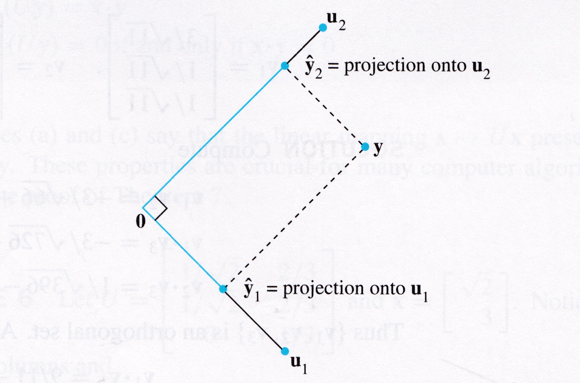
For example, let’s take the case where \(\mathbf{y} \in \mathbb{R}^2.\)
Let’s say we are given \(\mathbf{u}_1, \mathbf{u}_2\) such that \(\mathbf{u}_1\) is orthogonal to \(\mathbf{u}_2\), and so together they span \(\mathbb{R}^2.\)
Then \(\mathbf{y}\) can be written in the form
The first term is the projection of \(\mathbf{y}\) onto the subspace spanned by \(\mathbf{u}_1\) and the second term is the projection of \(\mathbf{y}\) onto the subspace spanned by \(\mathbf{u}_2.\)
So this equation expresses \(\mathbf{y}\) as the sum of its projections onto the (orthogonal) axes determined by \(\mathbf{u}_1\) and \(\mathbf{u}_2\).
This is an useful way of thinking about coordinates in an orthogonal basis: coordinates are projections onto the axes!
# image credit: Lay 4th edition figure 4 in Ch 6.2
display(Image("images/Lay-fig-6-2-4.jpg", width=600))
Question Time! Q21.3
Orthonormal Sets
Orthogonal sets are therefore very useful. However, they become even more useful if we normalize the vectors in the set.
A set \(\{\mathbf{u}_1,\dots,\mathbf{u}_p\}\) is an orthonormal set if it is an orthogonal set of unit vectors.
If \(W\) is the subspace spanned by such as a set, then \(\{\mathbf{u}_1,\dots,\mathbf{u}_p\}\) is an orthonormal basis for \(W\) since the set is automatically linearly independent.
The simplest example of an orthonormal set is the standard basis \(\{\mathbf{e}_1, \dots,\mathbf{e}_n\}\) for \(\mathbb{R}^n\).
Pro tip: keep the terms clear in your head:
orthogonal is (just) perpendicular, while
orthonormal is perpendicular and unit length.
(You can see the word “normalized” inside “orthonormal”).
Orthogonal Mappings
Matrices with orthonormal columns are particularly important.
Theorem. A \(m\times n\) matrix \(U\) has orthonormal columns if and only if \(U^TU = I\).
Proof. Let us suppose that \(U\) has only three columns which are each vectors in \(\mathbb{R}^m\) (but the proof will generalize to \(n\) columns).
Let \(U = [\mathbf{u}_1\;\mathbf{u}_2\;\mathbf{u}_3].\) Then:
The columns of \(U\) are orthogonal if and only if
The columns of \(U\) all have unit length if and only if
So \(U^TU = I.\)
Orthonormal Matrices Preserve Length and Orthogonality
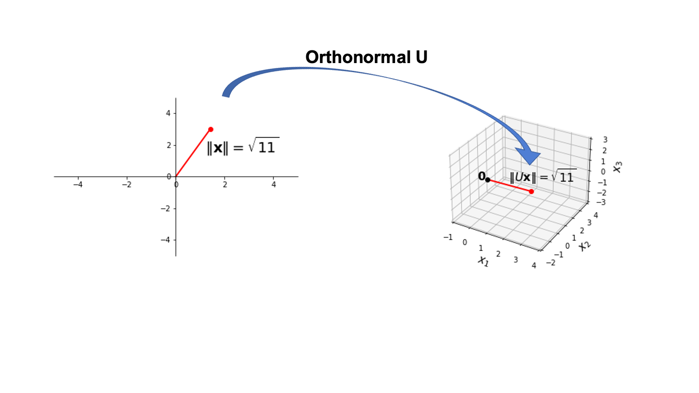
Theorem. Let \(U\) by an \(m\times n\) matrix with orthonormal columns, and let \(\mathbf{x}\) and \(\mathbf{y}\) be in \(\mathbb{R}^n.\) Then:
\(\Vert U\mathbf{x}\Vert = \Vert\mathbf{x}\Vert.\)
\((U\mathbf{x})^T(U\mathbf{y}) = \mathbf{x}^T\mathbf{y}.\)
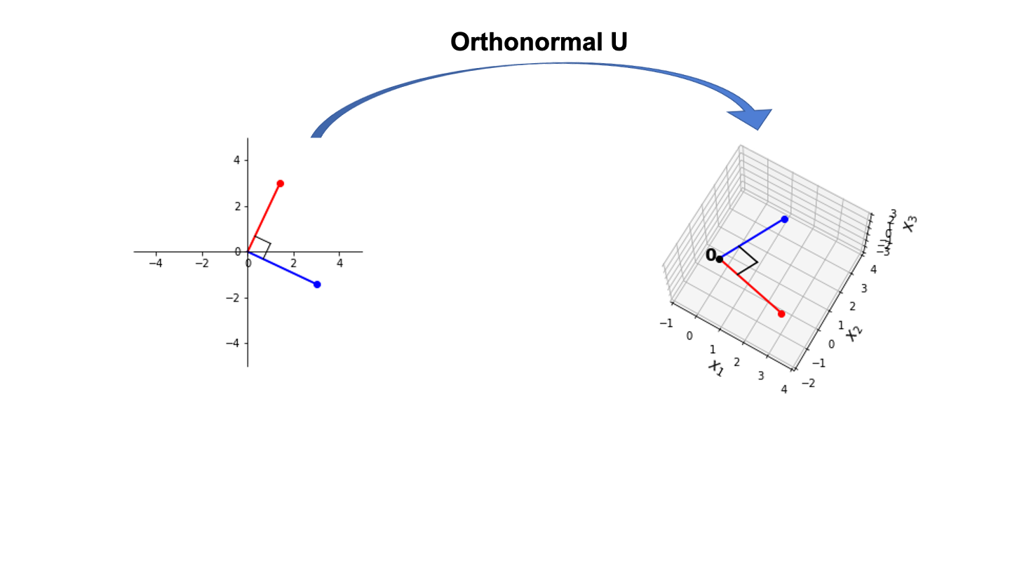
\((U\mathbf{x})^T(U\mathbf{y}) = 0\;\mbox{if and only if}\; \mathbf{x}^T\mathbf{y} = 0.\)
Properties 1. and 3. make an important statement.
So, viewed as a linear operator, an orthonormal matrix is very special: the lengths of vectors, and therefore the distances between points is not changed by the action of \(U\).
Notice as well that \(U\) is \(m \times n\) – it may not be square.
So it may map vectors from one vector space to an entirely different vector space – but the distances between points will not be changed!
# image source: Figure Components.ipynb + Lecture 21 Figures.pptx
display(Image("images/L21 F1.png", width=800))
… and the orthogonality of vectors will not be changed!
# image source: Figure Components.ipynb + Lecture 21 Figures.pptx
display(Image("images/L21 F2.png", width=700))
Note however that we cannot in general construct an orthonormal map from a higher dimension to a lower one.
For example, three orthogonal vectors in \(\mathbb{R}^3\) cannot be mapped to three orthogonal vectors in \(\mathbb{R}^2\). Can you see why this is impossible? What is it about the definition of an orthonormal set that prevents this?
Example. Let \(U = \begin{bmatrix}1/\sqrt{2}&2/3\\1/\sqrt{2}&-2/3\\0&1/3\end{bmatrix}\) and \(\mathbf{x} = \begin{bmatrix}\sqrt{2}\\3\end{bmatrix}.\) Notice that \(U\) has orthonormal columns, and
Let’s verify that \(\Vert Ux\Vert = \Vert x\Vert.\)
When Orthonormal Matrices are Square
Finally, one of the most useful transformation matrices is obtained when the columns of the matrix are orthonormal…
… and the matrix is square.
These matrices map vectors in \(\mathbb{R}^n\) to new locations in the same space, ie, \(\mathbb{R}^n\).
… in a way that preserves lengths, distances and orthogonality.
Now, consider the case when \(U\) is square, and has orthonormal columns.
Then the fact that \(U^TU = I\) implies that \(U^{-1} = U^T.\)
Then \(U\) is called an orthogonal matrix.
A good example of an orthogonal matrix is a rotation matrix:
Using trigonometric identities, you should be able to convince yourself that
and hopefully you can visualize how \(R\) preserves lengths and orthogonality.