.ipynb .pdf

repository

Binder

Contents

Computer Graphics

# for QR codes use inline
%matplotlib inline
qr_setting = 'url'
#
# for lecture use notebook
# %matplotlib notebook
# qr_setting = None
#
%config InlineBackend.figure_format='retina'
# import libraries
import numpy as np
import matplotlib as mp
import pandas as pd
import matplotlib.pyplot as plt
import laUtilities as ut
import slideUtilities as sl
import demoUtilities as dm
import pandas as pd
from importlib import reload
from datetime import datetime
from IPython.display import Image
from IPython.display import display_html
from IPython.display import display
from IPython.display import Math
from IPython.display import Latex
from IPython.display import HTML
from IPython.display import YouTubeVideo
from IPython.display import Audio
reload(sl)
reload(ut);

Computer Graphics is the study of creating, synthesizing, manipulating, and using visual information in the computer.

Today we’ll study the mathematics behind computer graphics.

Recommended Textbook: Mathematics for 3D Game Programming and Computer Graphics, Third Edition

Motivation

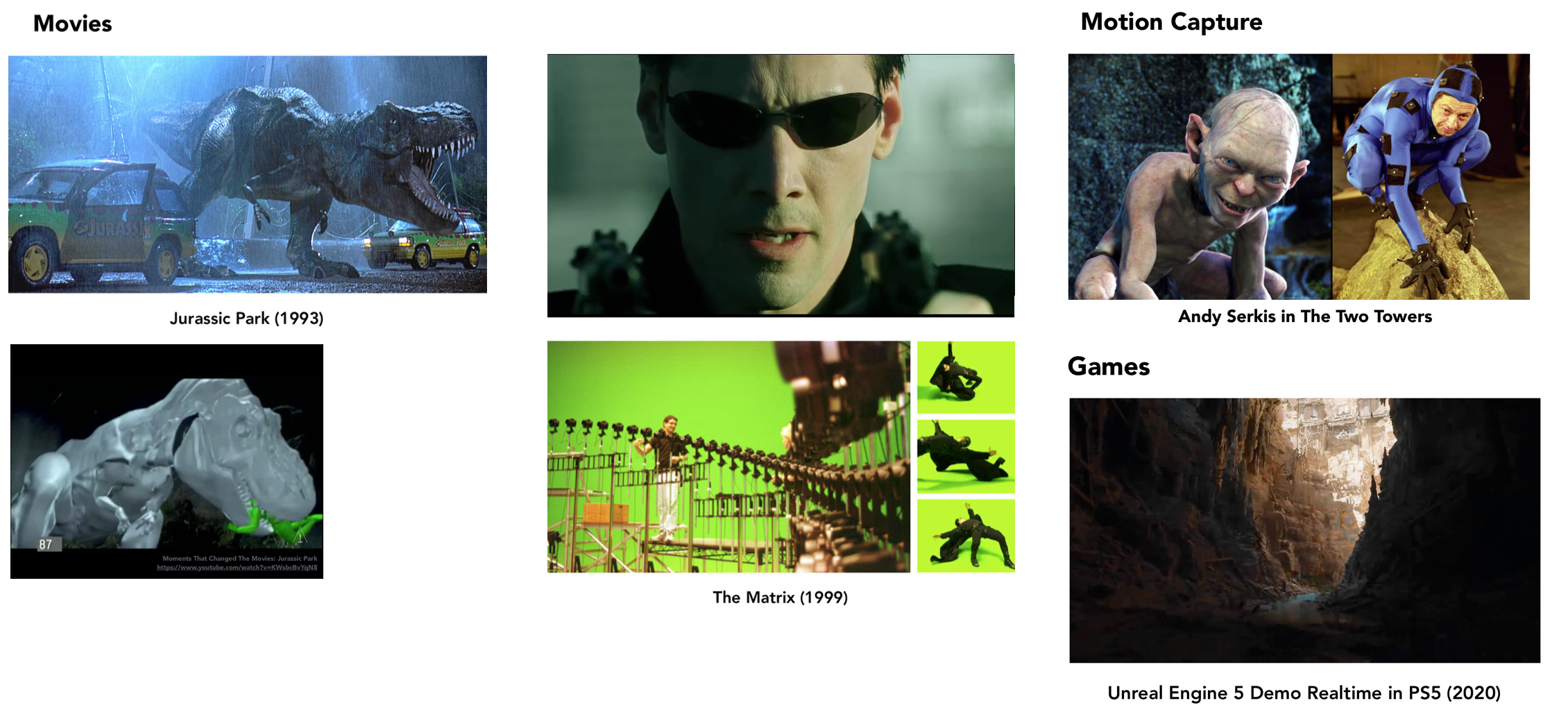
Entertaiment: film productions, film effects, motion capture, gaming

# Source: CS 184 Lecture Slides, UC Berkeley, Ng Ren
display(Image("images/ComputerGraphics/motivation-entertainment.png", width=900))

Science and Engineer: product design, visualization, computer-aided desingn

# Source: CS 184 Lecture Slides, UC Berkeley, Ng Ren
display(Image("images/ComputerGraphics/motivation-product-visual.png", width=750))

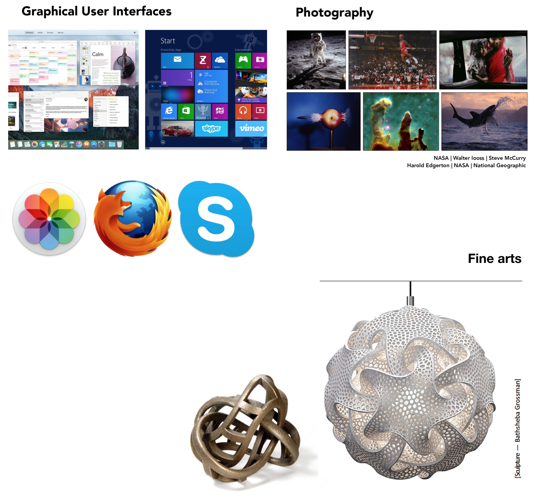
Graphic Arts: graphical user interface, digital photography, graphic design, fine arts

# Source: CS 184 Lecture Slides, UC Berkeley, Ng Ren; CS 680 Lecture Slides, Boston University, Emily Whiting
display(Image("images/ComputerGraphics/motivation-finearts.png", width=700))

Architectural design

Visual Simulation

Virtual Reality, Augmented Reality, 3D Printing

Transformations

We have talked about Geometric Linear Transformations of \(\mathbb{R}^2\):

1. Reflection over the \(x_1,x_2\) axes, over the lines \(x_2=x_1, x_2=-x_1\), and through the origin.

2. Horizontal and vertical expansion.

3. Horizontal and vertical shearing.

4. Projection onto the \(x_1,x_2\) axes.

Today, we will talk about 3D transformations and its applications.

In the application aspects, why are we studying transformation? Why 3D transformations?

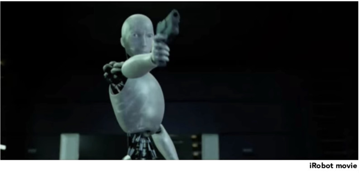
1. Tranform can describe position of object instances

display(Image("images/ComputerGraphics/robot01.png", width=750))

1. Transform can describe relative position of connected body part

display(Image("images/ComputerGraphics/robot02.png", width=750))

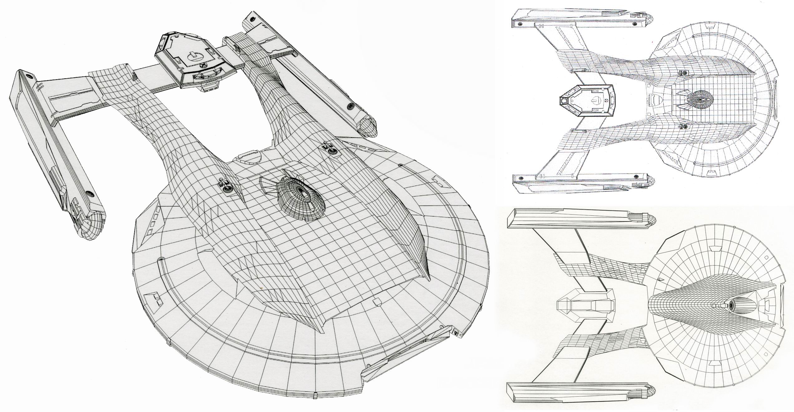
Jurassic Park movie: Behind the scene.

id='KWsbcBvYqN8'
display(YouTubeVideo(id=id, width=900, height=400))

The computer graphics seen in movies and videogames works in three stages:

1. A 3D model of the scene objects is created;

2. The model is converted into (many small) polygons in 3D that approximate the surfaces of the model; and

3. The polygons are transformed via a linear transformation to yield a 2D representation that can be shown on a flat screen.

There is interesting mathematics in each stage, but the transformations that take place in the third stage are linear, and that’s what we’ll study today.

# source http://vignette4.wikia.nocookie.net/memoryalpha/images/8/87/Akira_class_CGI_wireframe_model_by_ILM.jpg/revision/latest?cb=20130221104236&path-prefix=en
display(Image("images/ComputerGraphics/Akira_class_CGI_wireframe_model_by_ILM.jpg", width=750))

Initially, object models may be expressed in terms of smooth functions like polynomials.

However the first step is to convert those smooth functions into a set of discrete pieces – coordinates and line segments.

All subsequent processing is done in terms of the discrete coordinates that approximate the shape of the original model.

The reason for this conversion is that most transformations needed in graphics are linear.

Expressing the scene in terms of coordinates is equivalent to expressing it in terms of vectors, eg, in \(\mathbb{R}^3\).

And linear transformations on vectors are always matrix multiplications, so implementation is simple and uniform.

The resulting representation consists of lists of 3D coordinates called faces. Each face is a polygon.

The lines drawn between coordinates are implied by the way that coordinates are grouped into faces.

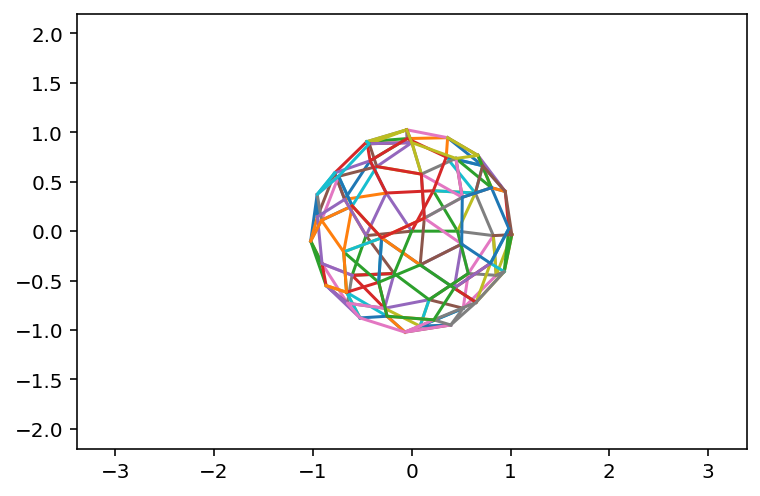
Example.

Here is a view of a ball-like object. It is centered at the origin.

The ball is represented in terms of 3D coordinates, but we are only plotting the \(x\) and \(y\) coordinates here.

Colors correspond to faces.

#
# load ball wireframe
import obj2clist as obj
with open('snub_icosidodecahedron.wrl','r') as fp:
    ball = obj.wrl2flist(fp)
#
# set up view
fig = plt.figure()
ax = plt.axes(xlim=(-5,5),ylim=(-5,5))
plt.plot(-2,-2,'')
plt.plot(2,2,'')
plt.axis('equal')
#
# plot the ball
for b in ball:
    ax.plot(b[0],b[1])

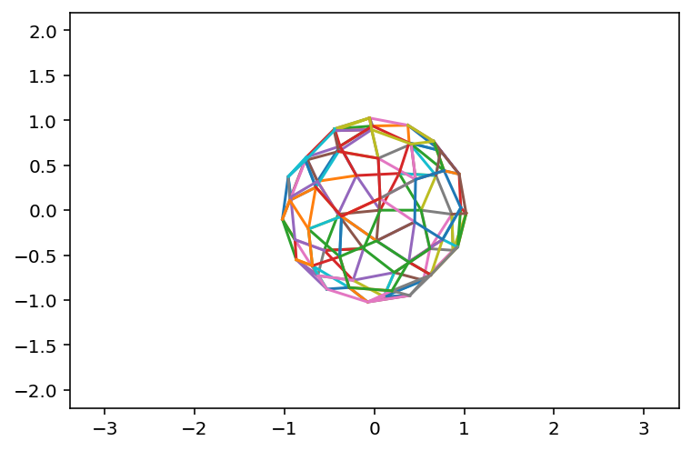
Rotation

Imagine that we want to circle the camera around the ball. This is equivalent to rotating the ball around the \(y\) axis. (See Maya Showcases)

This is a linear transformation. We can implement it by multiplying the coordinates of the ball by a rotation matrix. To define the rotation matrix, we need to think about what happens to each of the columns of \(I: {\bf e_1, e_2, e_3.}\)

To rotate through an angle of \(\alpha\) radians around the \(y\) axis,

the vector \({\bf e_1} = \left[\begin{array}{r}1\\0\\0\end{array}\right]\) goes to \(\left[\begin{array}{c}\cos \alpha\\0\\\sin \alpha\end{array}\right].\)

Of course, \({\bf e_2}\) is unchanged.

And \({\bf e_3} = \left[\begin{array}{r}0\\0\\1\end{array}\right]\) goes to \(\left[\begin{array}{c}-\sin \alpha\\0\\\cos \alpha\end{array}\right].\)

So the entire rotation matrix is:

\[\begin{split}\begin{bmatrix}\cos \alpha&0&-\sin \alpha\\0&1&0\\\sin \alpha&0&\cos\alpha\end{bmatrix}.\end{split}\]

# set up view
import matplotlib.animation as animation
mp.rcParams['animation.html'] = 'jshtml'

fig = plt.figure()
ax = plt.axes(xlim=(-5,5),ylim=(-5,5))
plt.plot(-2,-2,'')
plt.plot(2,2,'')
plt.axis('equal')
ballLines = []
for b in ball:
    ballLines += ax.plot([],[])
#
#to get additional args to animate:
#def animate(angle, *fargs):
#    fargs[0].view_init(azim=angle)
def animate(frame):
    angle = 2.0 * np.pi * (frame/100.0)
    rotationMatrix = np.array([[np.cos(angle), 0, -np.sin(angle)],
                               [0,             1,              0],
                               [np.sin(angle), 0, np.cos(angle)]])
    for b,l in zip(ball,ballLines):
        rb = rotationMatrix @ b
        l.set_data(rb[0],rb[1])
    fig.canvas.draw()
#
# create the animation 
animation.FuncAnimation(fig, animate,
                       frames=np.arange(0,100,1),
                       fargs=None,
                       interval=100,
                       repeat=False)

Once Loop Reflect

Translation

Manipulating graphics objects using matrix multiplication is very convenient.

However, there is a common operation that is not a linear transformation: translation – that is, motion.

Remember that a transformation \(T(x)\) is linear if \(T(x + y) = T(x) + T(y)\) and \(T(cx) = cT(x)\).

If \(T(x)\) is a translation, then \(T(x) = x + b\) for some \(b\).

But then \(T(x + y) \neq T(x) + T(y)\).

There is a nice way to avoid this difficulty, while keeping things linear.

We will use what are called homogeneous coordinates.

That is, adding another coordinate

We identify each point \(\left[\begin{array}{r}x\\y\\z\end{array}\right] \in \mathbb{R}^3\) with a corresponding point \(\left[\begin{array}{r}x\\y\\z\\1\end{array}\right] \in \mathbb{R}^4.\)

The coordinates of the point in \(\mathbb{R}^4\) are the homogeneous coordinates for the point in \(\mathbb{R}^3.\)

The extra component gives us a constant that we can scale and add to the other coordinates, as needed, via matrix multiplication.

This means for 3D graphics, all transformation matrices are \(4\times 4.\)

Example.

Let’s say we want to move a point \((x, y, z)\) to location \((x+h, y+k, z+m).\)

We represent the point in homogeneous coordinates as \(\left[\begin{array}{r}x\\y\\z\\1\end{array}\right].\)

The transformation corresponding to this ‘translation’ is:

\[\begin{split}\left[\begin{array}{cccc}1&0&0&h\\0&1&0&k\\0&0&1&m\\0&0&0&1\end{array}\right]\left[\begin{array}{r}x\\y\\z\\1\end{array}\right] = \left[\begin{array}{c}x+h\\y+k\\z+m\\1\end{array}\right].\end{split}\]

If we only consider \(x, y,\) and \(z\) this is not a linear transformation. But of course, in \(\mathbb{R}^4\) this most definitely is a linear transformation.

We have ‘sheared’ in the fourth dimension, which affects the other three. A very useful trick!

Constructing Matrices for Homogeneous Coordinates

For any transformation \(A\) that is linear in \(\mathbb{R}^3\) (such as scaling, rotation, reflection, shearing, etc.), we can construct the corresponding matrix for homogeneous coordinates quite simply:

If $\( A = \begin{bmatrix}\blacksquare&\blacksquare&\blacksquare\\\blacksquare&\blacksquare&\blacksquare\\\blacksquare&\blacksquare&\blacksquare\end{bmatrix}\)$

Then the corresponding transformation for homogeneous coordinates is:

\[\begin{split}\begin{bmatrix}\blacksquare&\blacksquare&\blacksquare&0\\\blacksquare&\blacksquare&\blacksquare&0\\\blacksquare&\blacksquare&\blacksquare&0\\0&0&0&1\end{bmatrix}\end{split}\]

In other words, when performing a linear transformation on \(x, y\), and \(z\), one simply ‘carries along’ the extra coordinate without modifying it.

Matrices for 3D Transforamtions

Scaling

\[\begin{split}\begin{bmatrix} s_x&0&0&0 \\ 0&s_y&0&0 \\0&0&s_z&0 \\0&0&0&1\end{bmatrix}\end{split}\]

Translation

\[\begin{split}\begin{bmatrix} 1&0&0&h\\0&1&0&k\\0&0&1&m\\0&0&0&1\end{bmatrix}\end{split}\]

Rotation around x-, y-, z- axis couterclockwise and looking towards the origin

\[\begin{split}R_x(\alpha)=\begin{bmatrix}1&0&0&0\\ 0&\cos \alpha&-\sin \alpha&0\\0&\sin \alpha&\cos\alpha&0\\0&0&0&1\end{bmatrix}.\end{split}\]

\[\begin{split}R_y(\alpha)=\begin{bmatrix}\cos \alpha&0&\sin \alpha&0\\0&1&0&0\\-\sin \alpha&0&\cos\alpha&0\\0&0&0&1\end{bmatrix}.\end{split}\]

\[\begin{split}R_z(\alpha)=\begin{bmatrix}\cos \alpha&-\sin \alpha&0&0\\\sin \alpha&\cos\alpha&0&0\\0&0&1&0\\0&0&0&1\end{bmatrix}.\end{split}\]

Perspective Projections

There is another nonlinear transformation that is important in computer graphics: perspective.

Happily, we will see that homogeneous coordinates allow us to capture this too as a linear transformation in \(\mathbb{R}^4\).

The eye, or a camera, captures light (essentially) in a single location, and hence gathers light rays that are converging.

So, to portray a scene with realistic appearance, it is necessary to reproduce this effect.

The effect can be thought of as “nearer objects are larger than further objects.” (Maya Showcases)

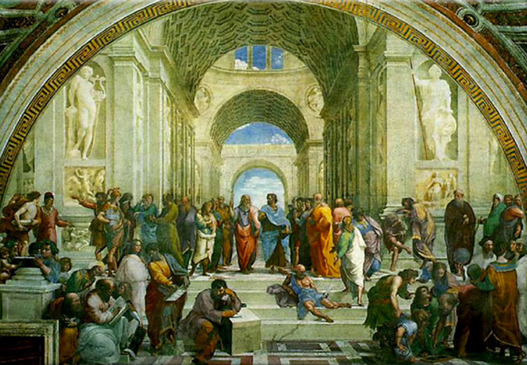
This was (re)discovered by Renaissance artists (supposedly first by Filippo Brunelleschi, around 1405).

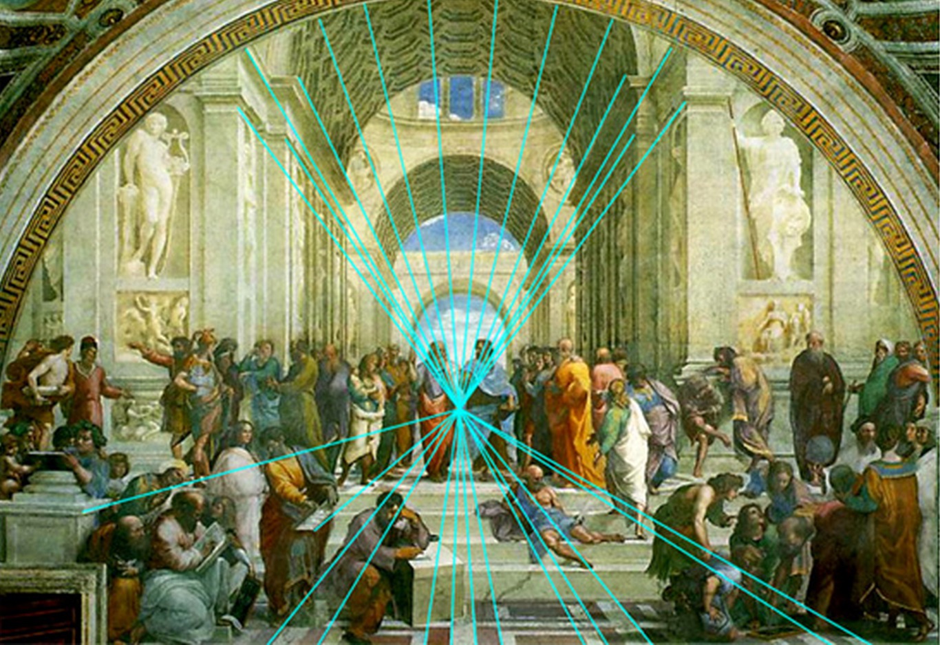
Here is a famous example: Raphael’s School of Athens (1510).

#source: http://www.webexhibits.org/sciartperspective/tylerperspective.html
display(Image("images/Raphael-SchoolofAthens.jpg", width=750))

display(Image("images/Raphael-SchoolofAthens-Perspective.jpg", width=750))

We now understand that this effect interacts in a powerful way with neural circuitry in our brains.

The mind reconstructs a sense of three dimensions from the two dimensional information presented to it by the retina.

This is done by sophisticated processing in the visual cortex, which is a fairly large portion of the brain.

# set up view
import matplotlib.animation as animation
mp.rcParams['animation.html'] = 'jshtml'

fig = plt.figure()
ax = plt.axes(xlim=(-5,5),ylim=(-5,5))
plt.plot(-2,-2,'')
plt.plot(2,2,'')
plt.axis('equal')
with open('cube.obj','r') as fp:
    cube = obj.obj2flist(fp)
cube = obj.homogenize(cube)
cubeLines = []
for c in cube:
    cubeLines += ax.plot([],[])
#
def animate(i):
    angle = 2.0 * np.pi * (i/100.0)
    P = np.array([[1.,0,0,0],[0,1.,0,0],[0,0,0,0],[0,0,-1./8,1]]).dot(np.array([[np.cos(angle),0,-np.sin(angle),0],[0,1,0,0],[np.sin(angle),0,np.cos(angle),0],[0,0,0,1]]))
    for b,l in zip(cube,cubeLines):
        rb = P.dot(b)
        l.set_data(rb[0]/rb[3],rb[1]/rb[3])
    fig.canvas.draw()
#
# create the animation 
animation.FuncAnimation(fig, animate,
                       frames=np.arange(0,100,1),
                       fargs=None,
                       interval=100,
                       repeat=False)

Once Loop Reflect

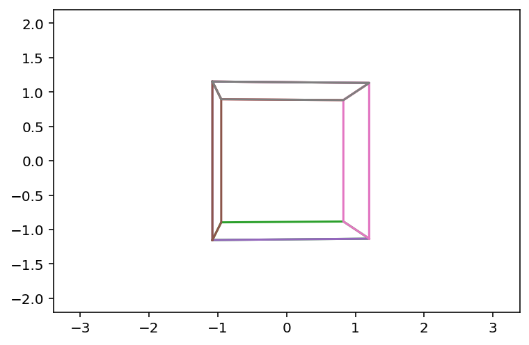
Notice that when the image is stationary, it appears flat (like a picture frame). As soon as it starts to move, it springs into 3D in perception.

Computing Perspective.

A standard setup for computing a perspective transformation is as shown in this figure:

# source: Lay, 4th edition
display(Image("images/Lay-fig-2-7-1.png", width=550))

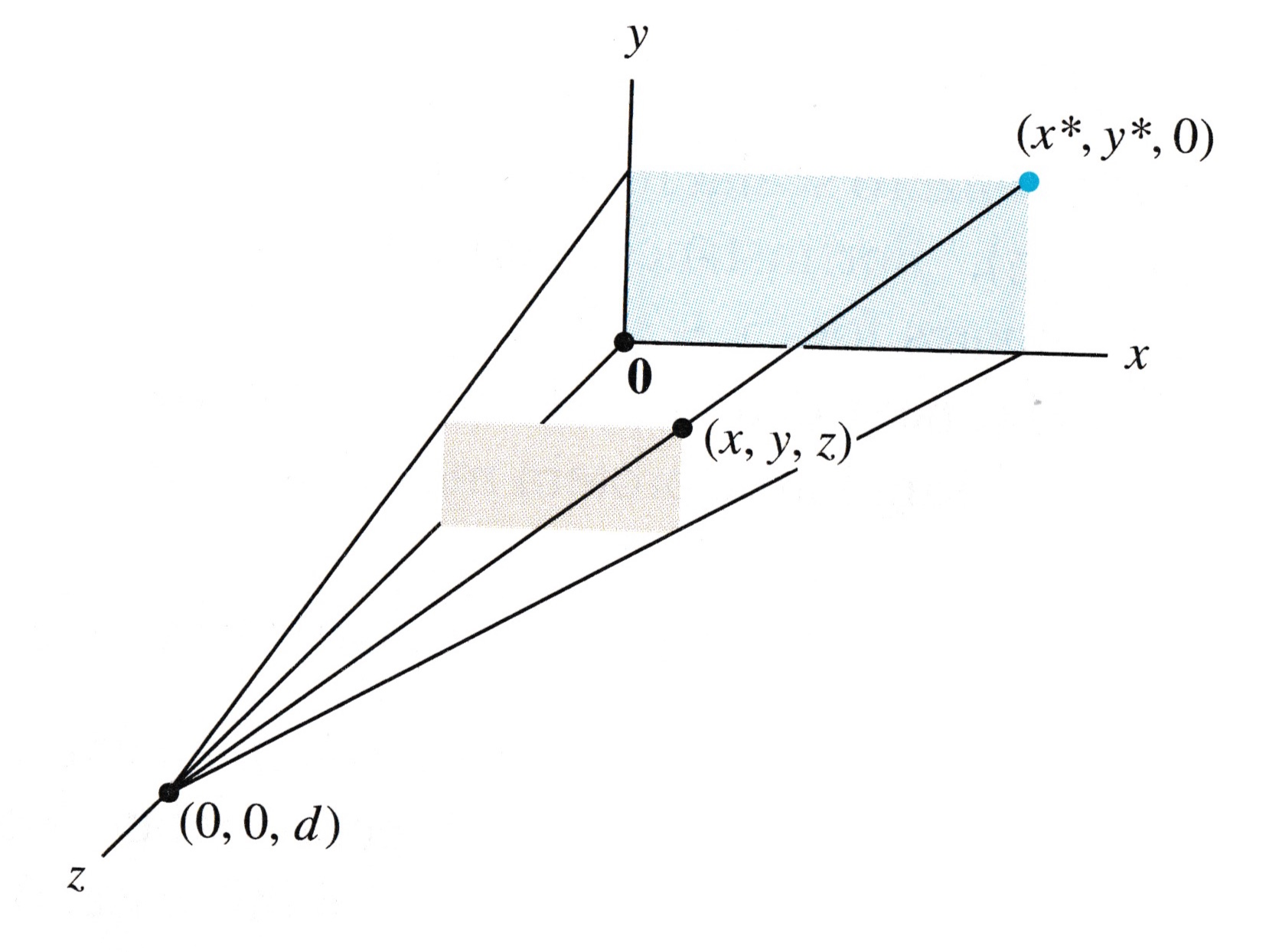
For simplicity, we will let the \(xy\)-plane represent the screen. This is called the viewing plane.

The eye/camera is located on the \(z\) axis, at the point \((0,0,d)\). This is call the center of projection.

A perspective projection maps each point \((x,y,z)\) onto an image point \((x^*,y^*,0)\) so that the center of projection and the two points are all on the same line.

# source: Lay, 4th edition
display(Image("images/Lay-fig-2-7-2.png", width=550))

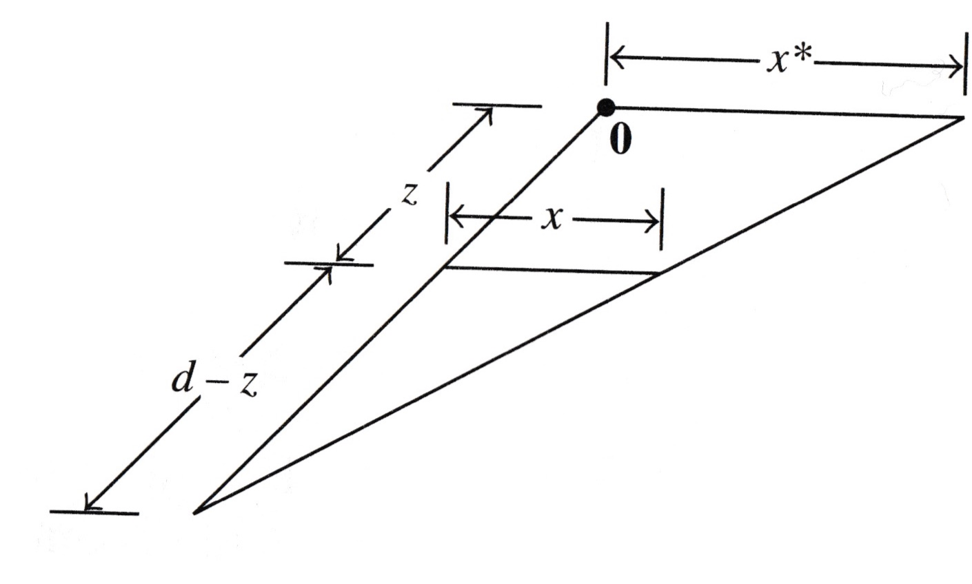
The way to compute the projection is using similar triangles.

The triangle in the \(xz\)-plane shows the lengths of corresponding line segments.

Similar triangles show that

\[\frac{x^*}{d} = \frac{x}{d-z}\]

and so

\[x^*=\frac{dx}{d-z}\;=\;\frac{x}{1-z/d}.\]

Notice that the function \(T: (x,z)\mapsto\frac{x}{1-z/d}\) is not linear.

Using homogeneous coordinates, we can construct a linear version of \(T\) in \(\mathbb{R}^4.\)

To do so, we establish the following convention: we will allow the fourth coordinate to vary away from 1.

However, when we plot, for a point \(\begin{bmatrix}x\\y\\z\\\end{bmatrix}\) we will plot the point \(\begin{bmatrix}\frac{x}{h}\\\frac{y}{h}\\\frac{z}{h}\end{bmatrix}.\)

In this way, by dividing the \(x,y,z\) coordinates by the \(h\) coordinate, we can implement a nonlinear transform in \(\mathbb{R}^3.\)

So, to implement the perspective transform, we want \(\begin{bmatrix}x\\y\\z\\1\end{bmatrix}\) to map to \(\begin{bmatrix}\frac{x}{1-z/d}\\\frac{y}{1-z/d}\\0\\1\end{bmatrix}.\)

The way we will implement this is to actually cause it to map to \(\begin{bmatrix}x\\y\\0\\1-z/d\end{bmatrix}.\)

Then, when we plot (dividing \(x\) and \(y\) by the \(h\) value) we will get the proper transform.

The matrix that implements this transformation is quite simple:

\[\begin{split}\begin{bmatrix}1&0&0&0\\0&1&0&0\\0&0&0&0\\0&0&-1/d&1\end{bmatrix}.\end{split}\]

So:

\[\begin{split}\begin{bmatrix}1&0&0&0\\0&1&0&0\\0&0&0&0\\0&0&-1/d&1\end{bmatrix}\begin{bmatrix}x\\y\\z\\1\end{bmatrix} = \begin{bmatrix}x\\y\\0\\1-z/d\end{bmatrix}.\end{split}\]

Composing Transformations

One big payoff for casting all graphics operations as linear transformations comes in the composition of transformations.

Consider two linear transformations \(T\) and \(S\). For example, \(T\) could be a scaling and \(S\) could be a rotation. Assume \(S\) is implemented by a matrix \(A\) and \(T\) is implemented by a matrix \(B\).

To first scale and then rotate a vector \(\mathbf{x}\) we would compute \(S(T(\mathbf{x}))\).

Of course this is implemented as \(A(B\mathbf{x}).\)

But note that this is the same as \((AB)\mathbf{x}.\) In other words, \(AB\) is a single matrix that both scales and rotates \(\mathbf{x}\).

By extension, we can combine any arbitrary sequence of linear transformations into a single matrix. This greatly simplifies high-speed graphics.

Note though that if \(C = AB\), then \(C\) is the transformation that first applies \(B\), then applies \(A\) (order matters).

Example. Let’s work in homogenous coordinates for points in \(\mathbb{R}^2\). Find the \(3\times 3\) matrix that corresponds to the composite transformation of first scaling by 0.3, then rotation of 90\(^\circ\) about the origin, and finally a translation of \(\begin{bmatrix}-0.5\\2\end{bmatrix}\) to each point of a figure.

# set up view
fig = plt.figure()
ax = plt.axes(xlim=(-5,5),ylim=(-5,5))
plt.plot(-2,-2,'')
plt.plot(2,2,'')
plt.axis('equal')
tri = np.array([[0.,1,-1,0],[1,-1,-1,1],[1,1,1,1]])
plt.plot(tri[0]/tri[2],tri[1]/tri[2],'b',label='X')
scale = np.array([[.3,0,0],[0,.3,0],[0,0,1]])
rotate = np.array([[0,-1.,0],[1,0,0],[0,0,1]])
translate = np.array([[1,0,-0.5],[0,1,2],[0,0,1]])
newtri = scale.dot(tri)
plt.plot(newtri[0]/newtri[2],newtri[1]/newtri[2],'r',label='S(X)')
newtri = rotate.dot(scale).dot(tri)
plt.plot(newtri[0]/newtri[2],newtri[1]/newtri[2],'g',label='R(S(X))')
newtri = translate.dot(rotate).dot(scale).dot(tri)
plt.plot(newtri[0]/newtri[2],newtri[1]/newtri[2],'y',label='T(R(S(X)))')
plt.legend();

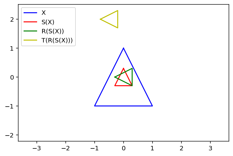
The scaling matrix is:

\[\begin{split}S = \begin{bmatrix}0.3&0&0\\0&0.3&0\\0&0&1\end{bmatrix}\end{split}\]

The rotation matrix is:

\[\begin{split}R = \begin{bmatrix}0&-1&0\\1&0&0\\0&0&1\end{bmatrix}\end{split}\]

(Note that \(\sin 90^\circ = 1\) and \(\cos 90^\circ = 0.\))

The translation matrix is:

\[\begin{split}T = \begin{bmatrix}1&0&-0.5\\0&1&2\\0&0&1\end{bmatrix}\end{split}\]

So the matrix for the composite transformation is:

\[\begin{split}TRS = \begin{bmatrix}1&0&-0.5\\0&1&2\\0&0&1\end{bmatrix}\begin{bmatrix}0&-1&0\\1&0&0\\0&0&1\end{bmatrix}\begin{bmatrix}0.3&0.3&0\\0&0.3&0\\0&0&1\end{bmatrix} = \begin{bmatrix}0&-0.3&-0.5\\0.3&0&2\\0&0&1\end{bmatrix}.\end{split}\]

Note that \(TRS\) would first apply S (scaling), then apply R (rotation), and last apply T (translation).

We need to be careful with the order of the matrices.

Consider a vector \(\mathbf{x}\in \mathbb{R}^2\). Let \(P\) be projection matrix that projects \(\mathbf{x}\) onto the x-axis and \(R\) be a rotation matrix that rotates \(\mathbf{x}\) by 30\(^\circ\) about the origin. Note that \(PR \ne RP\) where \(PR\) first rotate the vector and then apply projection while \(RP\) first projects the vector and then apply rotation.

Homework 7

Homework 7 will allow you to explore these ideas by computing various transformation matrices. I will give you some 3D wireframe objects and you will compute the necessary matrices to create a simple animation.

Here is what your finished product will look like:

import base64
VIDEO_TAG = """<video controls>
 <source src="data:video/x-m4v;base64,{0}" type="video/mp4">
 Your browser does not support the video tag.
</video>"""
def display_saved_anim(fname):
    with open(fname,'rb') as f:
        video = f.read()
    return HTML(VIDEO_TAG.format(base64.b64encode(video).decode('utf-8')))
display_saved_anim('images/hwk7Solution.mp4')

Application

Physics Based Simulation

We use physics-based simulation to capture the real world phenomena.

By physices-based simulation, we often think about fluid, hair, cloth, etc.

Cloth Simulation

There are different methods to animate cloth.

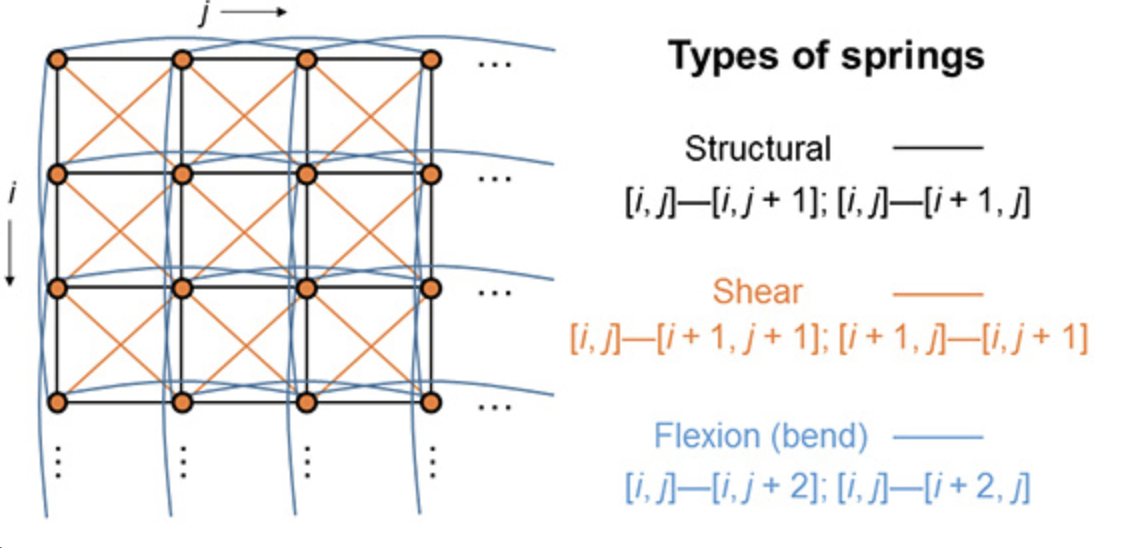
Mass Spring System

We consider the cloth as a collection of particles interconnected with different types of springs to behave bending, shearing, etc. And Hooke’s Law and Newton’s 2nd Law are used as the equations of motion to capture the cloth behaviors.

display(Image("images/ComputerGraphics/spring.png", width=750))

id='ib1vmRDs8Vw'
display(YouTubeVideo(id=id, width=900, height=400))

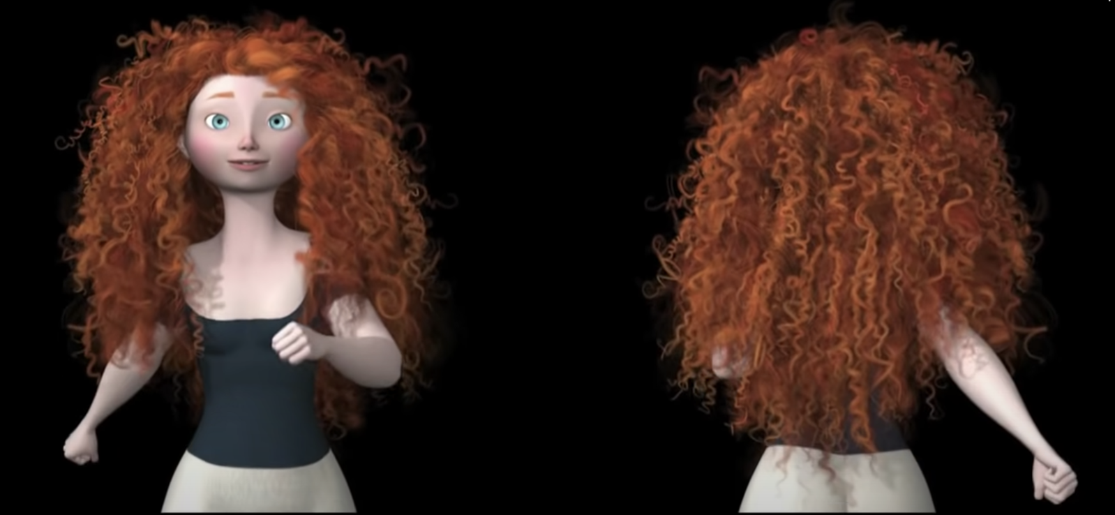
Hair Simulation

Images copyright @ Pixar

display(Image("images/ComputerGraphics/hair.png", width=750))

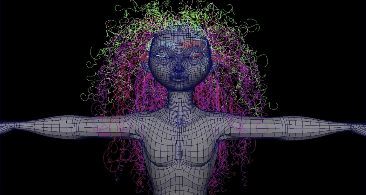
display(Image("images/ComputerGraphics/hair-render.png", width=750))

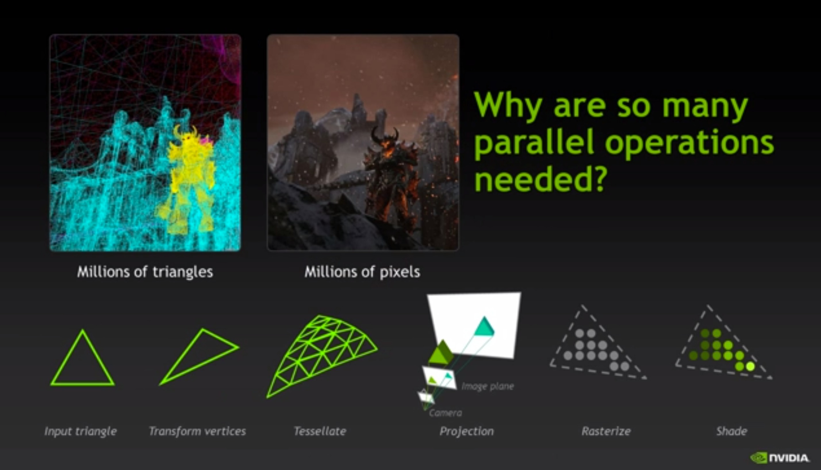
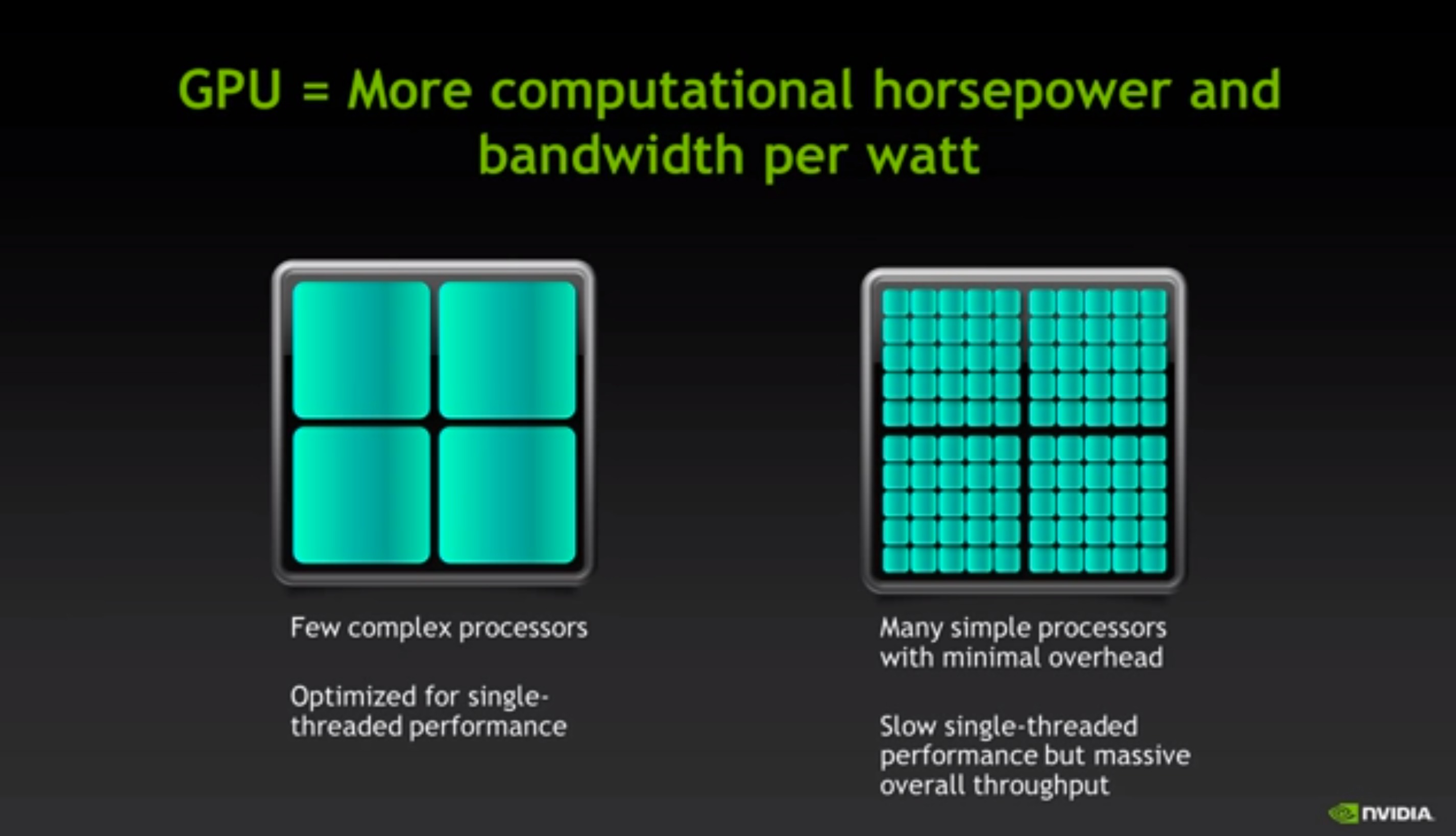
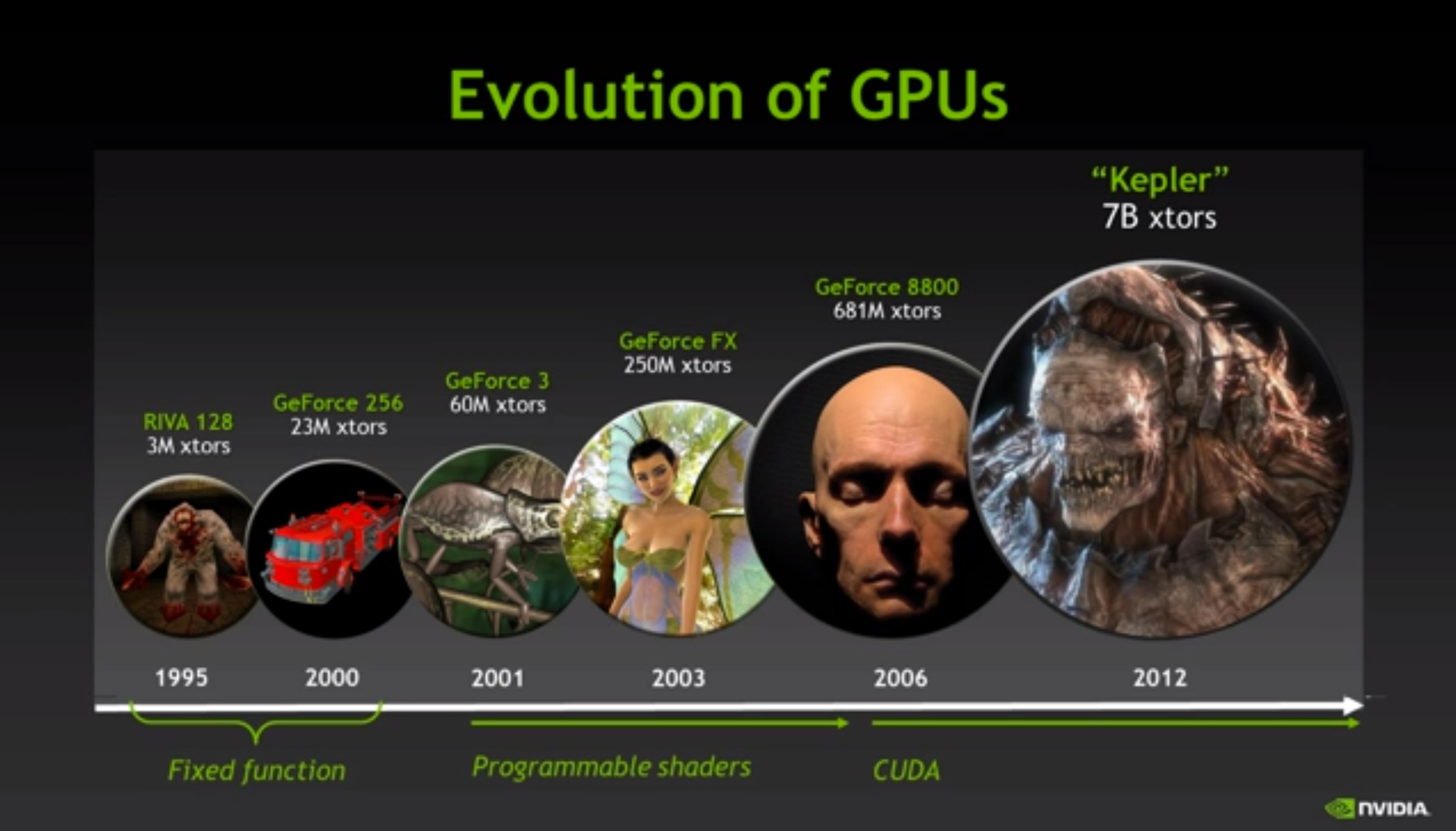
Fast Computation of Linear Systems using Graphics Processing Units (GPUs)

# Note: Another good source is http://pixeljetstream.blogspot.de/2015/02/life-of-triangle-nvidias-logical.html

# source http://on-demand.gputechconf.com/gtc/2013/video/S3424-Unlikely-Symbiosis-HPC-And-Gaming.mp4
display(Image("images/ComputerGraphics/Triangle-Processing.jpg", width=550))

# source http://on-demand.gputechconf.com/gtc/2013/video/S3424-Unlikely-Symbiosis-HPC-And-Gaming.mp4
display(Image("images/ComputerGraphics/CPU-GPU-Comparison.jpg", width=550))

# source http://on-demand.gputechconf.com/gtc/2013/video/S3424-Unlikely-Symbiosis-HPC-And-Gaming.mp4
display(Image("images/ComputerGraphics/GPU-Transistor-Scaling.jpg", width=550))

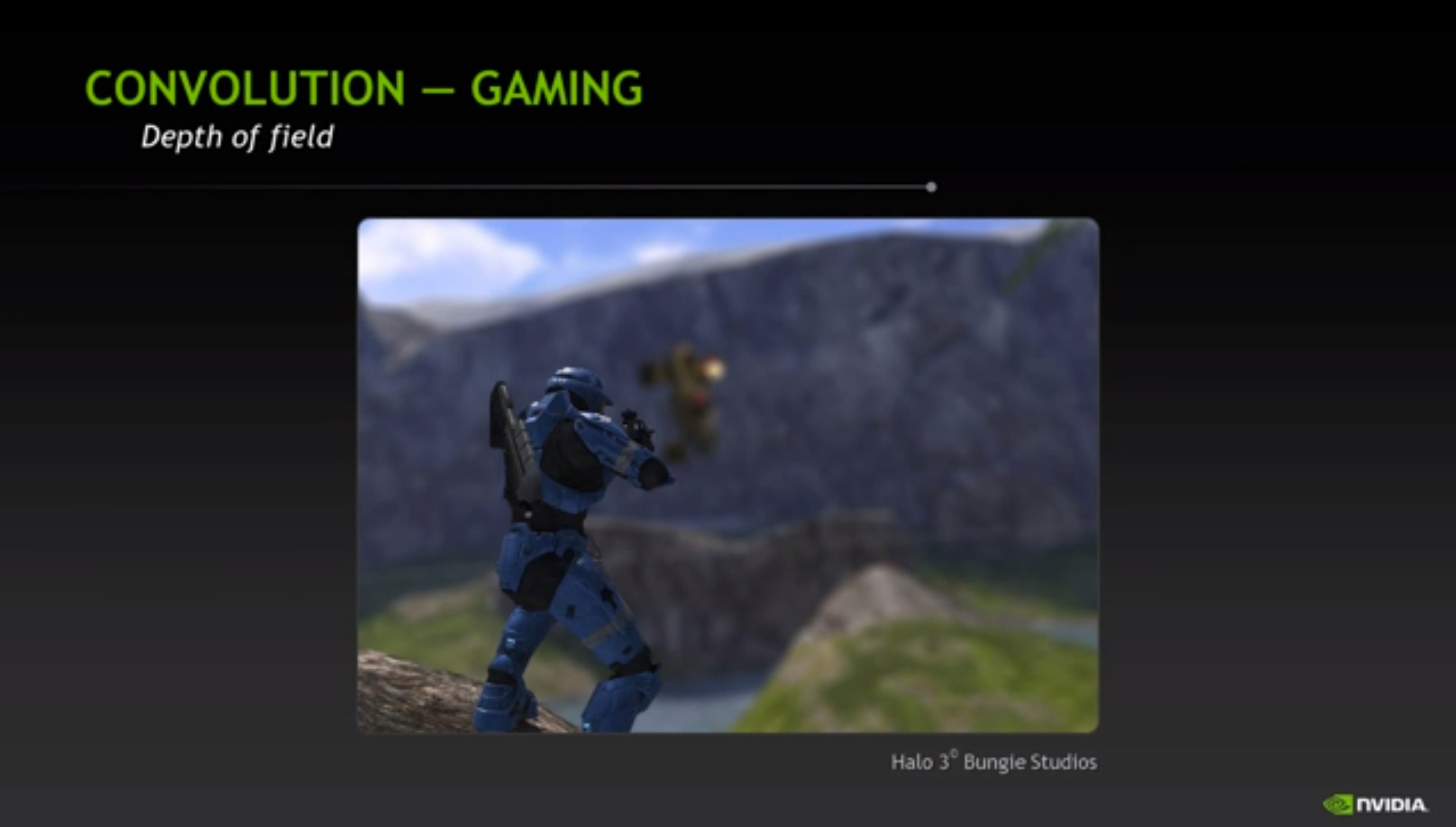
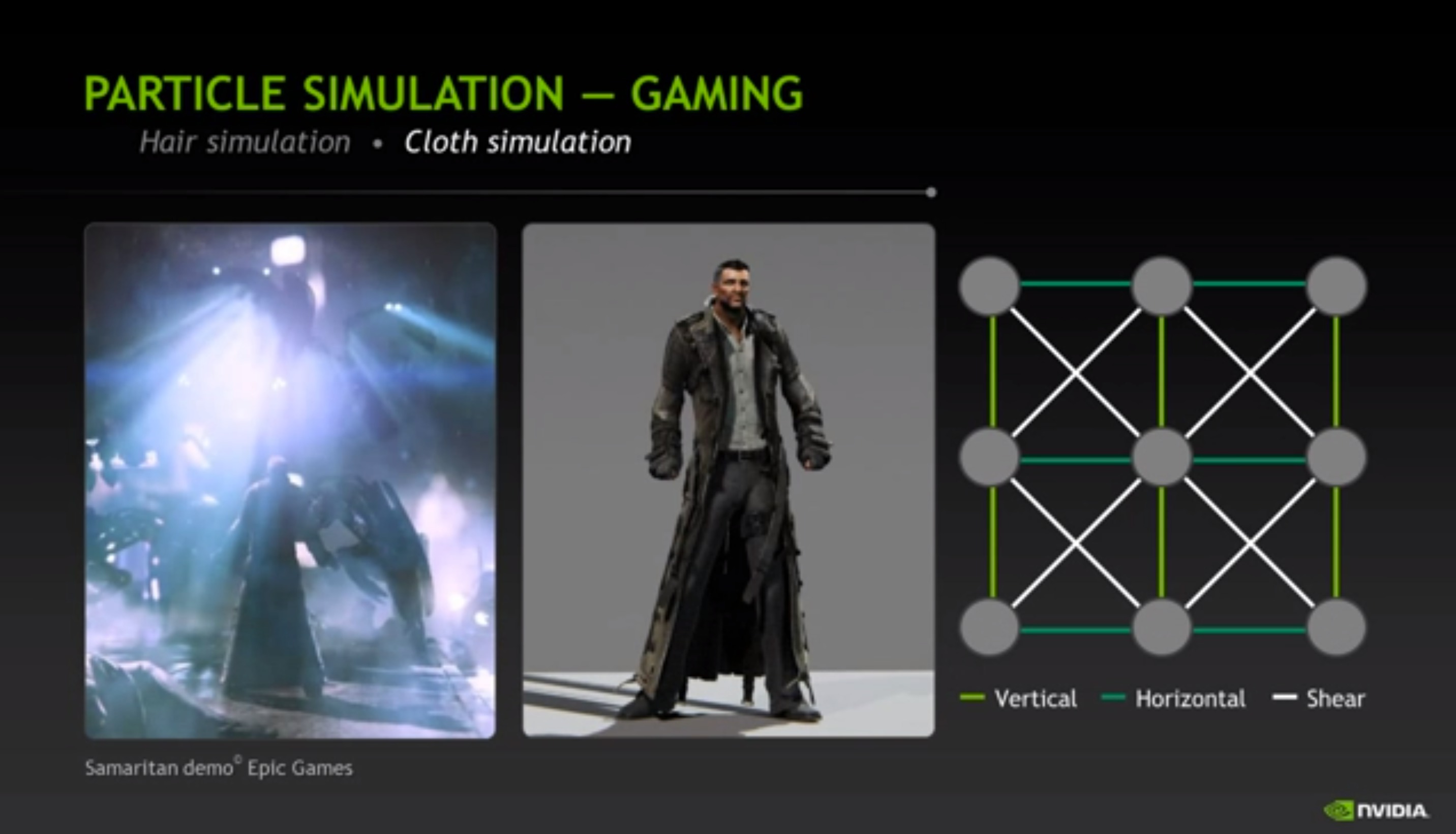
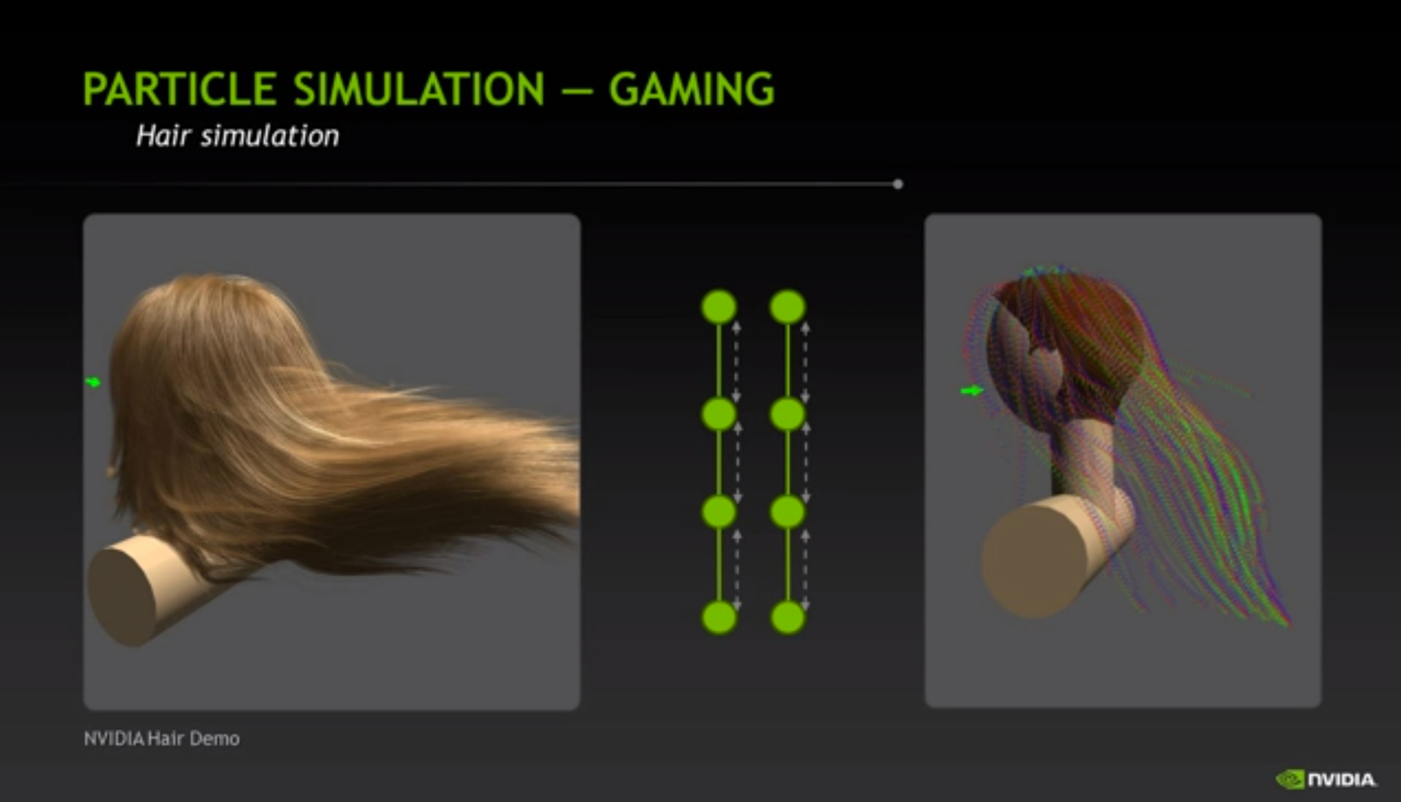
Examples of Other Linear Systems Used in Computer Graphics

# source http://on-demand.gputechconf.com/gtc/2013/video/S3424-Unlikely-Symbiosis-HPC-And-Gaming.mp4
display(Image("images/ComputerGraphics/Cloth-Simulation.jpg", width=550))

# source http://on-demand.gputechconf.com/gtc/2013/video/S3424-Unlikely-Symbiosis-HPC-And-Gaming.mp4
display(Image("images/ComputerGraphics/Hair-Simulation.jpg", width=550))

# source http://on-demand.gputechconf.com/gtc/2013/video/S3424-Unlikely-Symbiosis-HPC-And-Gaming.mp4
display(Image("images/ComputerGraphics/Convolution-Diagram.jpg", width=550))

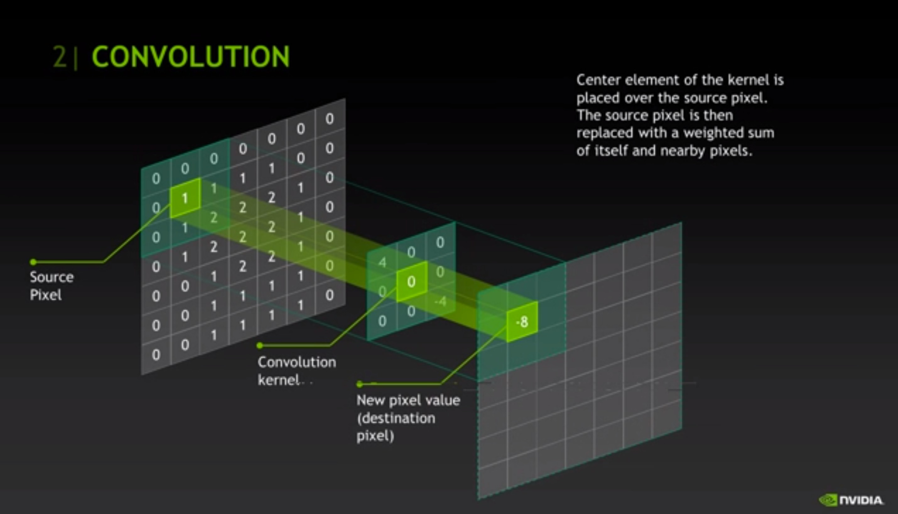
# source http://on-demand.gputechconf.com/gtc/2013/video/S3424-Unlikely-Symbiosis-HPC-And-Gaming.mp4
display(Image("images/ComputerGraphics/Convolution-Image-Example.jpg", width=550))

Matrix Factorizations Subspaces