\(A{\bf x} = {\bf b}\)
# for QR codes use inline
# %matplotlib inline
# qr_setting = 'url'
# qrviz_setting = 'show'
#
# for lecture use notebook
%matplotlib inline
qr_setting = None
#
%config InlineBackend.figure_format='retina'
# import libraries
import numpy as np
import matplotlib as mp
import pandas as pd
import matplotlib.pyplot as plt
import laUtilities as ut
import slideUtilities as sl
import demoUtilities as dm
import pandas as pd
from importlib import reload
from datetime import datetime
from IPython.display import Image
from IPython.display import display_html
from IPython.display import display
from IPython.display import Math
from IPython.display import Latex
from IPython.display import HTML;
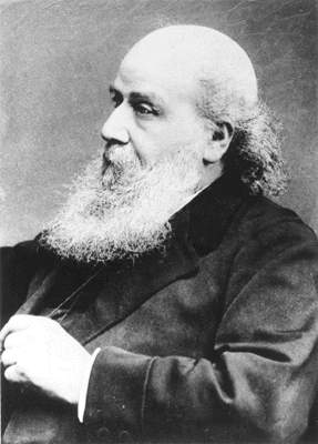
display(Image("images/James_Joseph_Sylvester.jpg", height = 400))
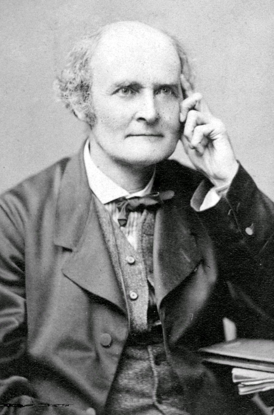
display(Image("images/Arthur_Cayley.jpg", width = 250))
HTML(u'Hamilton photo from:<a href="https://en.wikipedia.org/wiki/en:Image:Untitled04.jpg" class="extiw" title="w:en:Image:Untitled04.jpg">http://en.wikipedia.org/wiki/Image:Untitled04.jpg</a>, Public Domain, <a href="https://commons.wikimedia.org/w/index.php?curid=268041">Link</a>')
HTML(u'Cayley photo by <a href="https://en.wikipedia.org/wiki/Herbert_Rose_Barraud" class="extiw" title="en:Herbert Rose Barraud">Herbert Beraud</a> (1845–1896) - <a rel="nofollow" class="external free" href="http://www-groups.dcs.st-and.ac.uk/~history/PictDisplay/Cayley.html">http://www-groups.dcs.st-and.ac.uk/~history/PictDisplay/Cayley.html</a>, Public Domain, <a href="https://commons.wikimedia.org/w/index.php?curid=904674">Link</a>.')
Although ways of solving linear systems were known to the ancient Chinese, the 8th century Arabs, and were used to great effect by Gauss in the 1790s, the idea that the information content of a linear system should be captured in a matrix was not developed until J.J. Hamilton in 1850. He gave it the term matrix because he saw it as a sort of “womb” out of which many mathematical objects could be delivered.
Even then, it took a long time for the concept to emerge that one might want to multiply using matrices – that a matrix was an algebraic object. It was not until 1855 that Arthur Cayley came up with the “right” definition of how to multiply using matrices – the one that we use today.
Multiplying a Matrix by a Vector
Last lecture we studied the vector equation:
We also talked about how one can form a matrix from a set of vectors:
In particular, if we have \(n\) vectors \({\bf a_1},{\bf a_2}, ..., {\bf a_n} \in \mathbb{R}^m,\) then \(A\) will be an \(m \times n\) matrix:
We’re going to express a vector equation in a new way. We are going to say that
is the same as:
where \(A = \left[\begin{array}{cccc}\begin{array}{c}\vdots\\\vdots\\{\bf a_1}\\\vdots\\\vdots\end{array}&\begin{array}{c}\vdots\\\vdots\\{\bf a_2}\\\vdots\\\vdots\end{array}&\dots&\begin{array}{c}\vdots\\\vdots\\{\bf a_n}\\\vdots\\\vdots\end{array}\\\end{array}\right]\) and \({\bf x} = \left[\begin{array}{c}x_1\\x_2\\\vdots\\x_n\end{array}\right].\)
What we have done is to define Matrix-vector multiplication.
That is, \(A{\bf x}\) denotes multiplying a matrix and a vector, and we define it to be the same as a linear combination of the \(\{\bf a_1, a_2, \dots, a_n\}\) with weights \(x_1, x_2, \dots, x_n.\)
Here is the definition:
If \(A\) is an \(m\times n\) matrix, with columns \(\bf a_1, a_2, \dots, a_n,\) and if \({\bf x} \in \mathbb{R}^n,\) then the product of \(A\) and \(\bf x\), denoted \(A{\bf x}\), is the linear combination of the columns of \(A\) using the corresponding entries in \(x\) as weights; that is,
Notice that if \(A\) is an \(m\times n\) matrix, then \({\bf x}\) must be in \(\mathbb{R}^n\) in order for this operation to be defined. That is, the number of columns of \(A\) must match the number of rows of \({\bf x}.\)
If the number of columns of \(A\) does not match the number of rows of \({\bf x}\), then \(A{\bf x}\) has no meaning.
Matrix-Vector Multiplication Example
Relationship to Span
For \({\bf v_1}, {\bf v_2}, {\bf v_3} \in \mathbb{R}^m,\) write the linear combination \(3{\bf v_1} + 5{\bf v_2} + 7{\bf v_3}\) as a matrix times a vector.
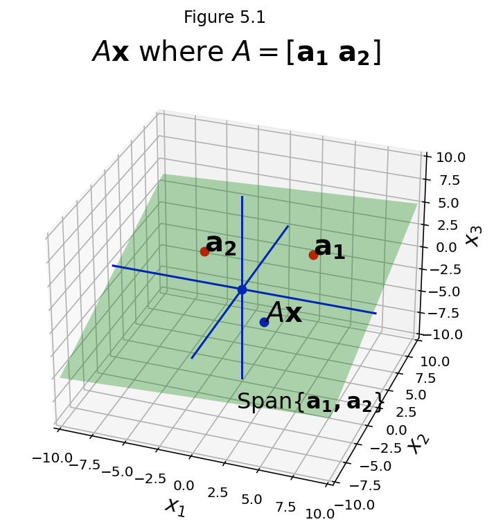
Notice that if \(A = [{\bf a_1} \; {\bf a_2} \; ... \;{\bf a_n}]\) then \(A{\bf x}\) is some point that lies in Span\(\{{\bf a_1},{\bf a_2}, \dots ,{\bf a_n}\}\).
fig = ut.three_d_figure((5, 1), 'Ax where A = [a1 a2]',
                        -10, 10, -10, 10, -10, 10, figsize=(9,6), qr=qr_setting)
v = [4.0,  4.0, 2.0]
u = [-4.0, 3.0, 1.0]
A = np.array([v, u]).T
x = np.array([-0.1, -0.75]).T
Ax = A @ x
fig.text(v[0], v[1], v[2], r'$\bf a_1$', 'a_1', size=20)
fig.text(u[0], u[1], u[2], r'$\bf a_2$', 'a_2', size=20)
fig.text(Ax[0], Ax[1], Ax[2], r'$A\bf x$', 'Ax', size=20)
fig.text(1, -4, -10, r'Span{$\bf a_1,a_2$}', 'Span{a_1, a_2}', size=16)
# fig.text(0.2, 0.2, -4, r'$\bf 0$', '0', size=20)
# plotting the span of v
fig.plotSpan(u, v, 'Green')
fig.plotPoint(u[0], u[1], u[2], 'r')
fig.plotPoint(v[0], v[1], v[2], 'r')
fig.plotPoint(0, 0, 0, 'b')
fig.plotPoint(Ax[0], Ax[1], Ax[2], 'b')
# plotting the axes
fig.plotIntersection([0,0,1,0], [0,1,0,0])
fig.plotIntersection([0,0,1,0], [1,0,0,0])
fig.plotIntersection([0,1,0,0], [1,0,0,0])
fig.set_title(r'$A{\bf x}$ where $A = \left[\bf a_1\;a_2\right]$',
              'Ax where A = [a_1 a_2]',
              size=20)
fig.ax.view_init(azim=290)
fig.save()
Question Time! Q5.1
The Matrix Equation
Now let’s write an equation. Let’s start with a linear system:
We saw last lecture that this linear system is equivalent to a vector equation, namely
Now, today we have learned that this vector equation is also equivalent to this matrix equation:
which has the form \(A{\bf x} = {\bf b}\).
Notice how simple it is to go from the linear system to the matrix equation: we put the coefficients of the linear system into \(A\), and the right hand side values into \({\bf b},\) and we can then write the matrix equation \(A{\bf x} = {\bf b}\) immediately.
OK, let’s write this out formally.
Theorem. If \(A\) is an \(m\times n\) matrix, with columns \(\bf a_1, a_2, \dots, a_n,\) and if \(\bf b\) is in \(\mathbb{R}^m\), the matrix equation
has the same solution set as the vector equation
which, in turn, has the same solution set as the system of linear equations whose augmented matrix is
This is an absolutely key result, because it gives us power to solve problems from three different viewpoints. If we are looking for a solution set \(x_1, x_2, \dots, x_n,\) there are three different questions we can ask:
What is the solution set of the linear system \([{\bf a_1} \; {\bf a_2} \; ... \;{\bf a_n}\;{\bf b}]\)?
What is the solution set of the vector equation \(x_1{\bf a_1} + x_2{\bf a_2} + ... + x_n{\bf a_n} = {\bf b}?\)
What is the solution set of the matrix equation \(A{\bf x} = {\bf b}?\)
We now know that all these questions have the same answer. And all of them can be solved by row reducing the augmented matrix \([{\bf a_1} \; {\bf a_2} \; ... \;{\bf a_n}\;{\bf b}].\)
In particular, one of the most common questions you will encounter is, given a matrix \(A\) and a vector \({\bf b}\), is there an \({\bf x}\) that makes \(A{\bf x} = {\bf b}\) true?
You will encounter this form of question quite often in fields like computer graphics, data mining, algorithms, or quantum computing.
Question Time! Q5.2
Existence of Solutions
We can see that \(A{\bf x} = {\bf b}\) has a solution if and only if \(\bf b\) is a linear combination of the columns of \(A\) – that is, if \(\bf b\) lies in Span\(\{{\bf a_1},{\bf a_2}, \dots ,{\bf a_n}\}.\) We can adopt the term “consistent” here too – i.e., is \(A{\bf x} = {\bf b}\) consistent?
Now we will ask a more general question, which is specifically about the matrix \(A\). That is:
Does \(A{\bf x} = {\bf b}\) have a solution for any \({\bf b}\)?
Example.
Let \(A = \left[\begin{array}{rrr}1&3&4\\-4&2&-6\\-3&-2&-7\end{array}\right]\) and \({\bf b} = \left[\begin{array}{r}b_1\\b_2\\b_3\end{array}\right].\) Is the equation \(A{\bf x} = {\bf b}\) consistent for all possible \(b_1, b_2, b_3?\)
We know how to test for consistency: form the augmented matrix and row reduce it.
The third entry in the column 4, simplified, is \(b_1 -\frac{1}{2}b_2+ b_3.\) This expression can be nonzero.
For example, take \(b_1 = 1, b_2 = 1, b_3 = 1;\) then the lower right entry is 1.5. This gives a row of the form \(0 = k\) which indicates an inconsistent system.
So the answer is “no, \(A{\bf x} = {\bf b}\) is not consistent for all possible \(b_1, b_2, b_3.\)”
Here is the echelon form of \(A\) (note we are talking only about \(A\) here, not the augmented matrix):
The equation \(A{\bf x} = {\bf b}\) fails to be consistent for all \(\bf b\) because the echelon form of \(A\) has a row of zeros.
If \(A\) had a pivot in all three rows, we would not care about the calculations in the augmented column because no matter what is in the augmented column, an echelon form of the augmented matrix could not have a row indicating \(0 = k\).
Question: OK, so \(A{\bf x} = {\bf b}\) is not always consistent. When is \(A{\bf x} = {\bf b}\) consistent?
Answer: When \(b_1 -\frac{1}{2}b_2+ b_3 = 0.\) This makes the last row of the augmented matrix all zeros.
This is a single equation in three unknowns, so it defines a plane through the origin in \(\mathbb{R}^3.\)
fig = ut.three_d_figure((5, 2), 'Ax where A = [a1 a2]',
                        -10, 10, -10, 10, -10, 10, figsize=(9,6), qr=qr_setting)
a1 = [1.0, -4.0, -3.0]
a2 = [3.0,  2.0, -2.0]
a3 = [4.0, -6.0, -7.0]
fig.text(a1[0], a1[1], a1[2], r'$\bf a_1$', 'a_1', size=20)
fig.text(a2[0], a2[1], a2[2], r'$\bf a_2$', 'a_2', size=20)
fig.text(a3[0], a3[1], a3[2], r'$\bf a_3$', 'a_3', size=20)
fig.text(0.2, 0.2, -4, r'$\bf 0$', '0', size=20)
fig.plotSpan(a1, a2, 'Green')
fig.plotPoint(a1[0], a1[1], a1[2], 'r')
fig.plotPoint(a2[0], a2[1], a2[2], 'r')
fig.plotPoint(a3[0], a3[1], a3[2], 'r')
fig.plotPoint(0, 0, 0, 'b')
fig.set_title(r'$b_1 - \frac{1}{2}b_2 + b_3 = 0$', size=20)
img = fig.save()
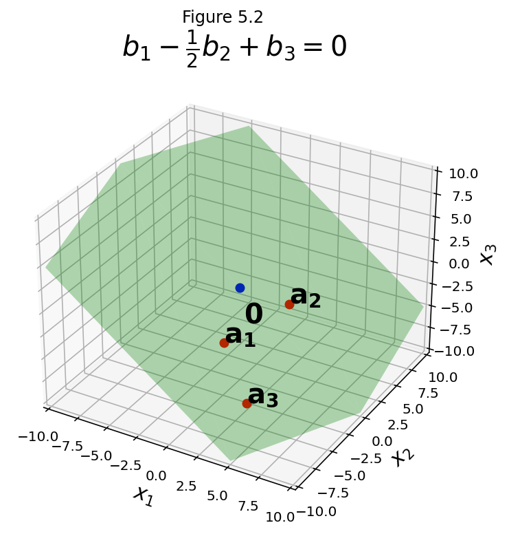
The set of points that makes \(b_1 - \frac{1}{2}b_2 + b_3 = 0\) is the set of \(\bf b\) values that makes \(A{\bf x} = {\bf b}\) consistent. But if \(A{\bf x} = {\bf b}\) then \({\bf b}\) lies within Span\(\{\bf a_1, a_2, a_3\}\).
So we have determined that Span\(\{\bf a_1, a_2, a_3\}\) is the same point set as \(b_1 - \frac{1}{2}b_2 + b_3 = 0\).
That means that Span\(\{\bf a_1, a_2, a_3\}\) is a plane in this case. In the figure we have plotted \(\bf a_1, a_2,\) and \(\bf a_3\) and you can see that all three points, as well as the origin, lie in the same plane.
Now, in the most general case, four points will not line in a plane. In other words, the span of three vectors in \(\mathbb{R}^3\) can be the whole space \(\mathbb{R}^3\).
Question Time! Q5.3
Now we will tie together all three views of our question.
Theorem: Let \(A\) be an \(m \times n\) matrix. Then the following statements are logically equivalent. That is, for a particular \(A,\) either they are all true or they are all false.
For each \(\bf b\) in \(\mathbb{R}^m,\) the equation \(A{\bf x} = {\bf b}\) has a solution.
Each \(\bf b\) in \(\mathbb{R}^m\) is a linear combination of the columns of \(A\).
The columns of \(A\) span \(\mathbb{R}^m\).
\(A\) has a pivot position in every row.
This theorem is very powerful and general.
Notice that we started by thinking about a matrix equation, but we ended by making statements about \(A\) alone.
This is the first time we are studying the property of a matrix itself; we will study many properties of matrices on their own as we progress.
Inner Product
There is a simpler way to compute the matrix-vector product. It uses a concept called the inner product or dot product.
The inner product is defined for two sequences of numbers, and returns a single number. For example, the expression
is the same as
which is the sum of the products of the corresponding entries, and yields the scalar value 5. This is the inner product of the two sequences.
The general definition of the inner product is:
Let’s see how this can be used to think about matrix-vector multiplication.
Consider the matrix-vector multiplication
Now, what is the first entry in the result? It is the inner product of the first row of \(A\) and \(\bf x\). That is,
This is a fast and simple way to compute the result of a matrix-vector product. Each element of the result is the inner product of the corresponding row of \(A\) and the vector \(\bf x\).
Example: Matrix-vector multiplication using Inner Products
Here we compute the same result as before, but now using inner products:
An (I)nteresting matrix
Consider this matrix equation:
This sort of matrix – with 1s on the diagonal and 0s everywhere else – is called an identity matrix and is denoted by \(I\).
You can see that for any \(\bf x\), \(I\bf x = x.\)
Algebraic Properties of the Matrix-Vector Product
We can now begin to lay out the algebra of matrices.
That is, we can define rules for valid symbolic manipulation of matrices.
Theorem. If \(A\) is an \(m \times n\) matrix, \(\bf u\) and \(\bf v\) are vectors in \(\mathbb{R}^n\), and \(c\) is a scalar, then:
\(A({\bf u} + {\bf v}) = A{\bf u} + A{\bf v};\)
\(A(c{\bf u}) = c(A{\bf u}).\)
Proof: Let us take \(n=3\), \(A = [\bf a_1\;a_2\;a_3],\) and \(\bf u,v \in \mathbb{R}^3.\)
Then to prove (1.):
And to prove (2.):