Diagonalization¶

# Source: http://img3.wikia.nocookie.net/__cb20140714004320/harrypotter/images/8/84/PottermoreDiagonAlley1.jpg
display(Image('images/PottermoreDiagonAlley1.jpg', width=450))
display(HTML('<b>"Welcome, Harry, to Diagon Alley"</b>'))
display(HTML('<b>-- Rubeus Hagrid</b>'))

"Welcome, Harry, to Diagon Alley"

-- Rubeus Hagrid

Today we consider an important factorization of a square matrix.

This factorization uses eigenvalues and eigenvectors, and makes many problems substantially easier.

Furthermore, it gives fundamental insight into the properties of a matrix.

Given a square matrix $A$, the factorization of $A$ is of the form

\[A = PDP^{-1}\]

where $D$ is a diagonal matrix.

Recall from last lecture, that the above equation means that $A$ and $D$ are similar matrices.

So this factorization amounts to finding a $P$ that allows us to make $A$ similar to a diagonal matrix.

This factorization allows us to

represent $A$ in a form that exposes the properties of $A$,
represent $A^k$ in an easy to use form, and
compute $A^k$ quickly for large values of $k$.

Let’s look at an example to show why this factorization is so important.

Powers of a Diagonal Matrix¶

Consider taking the powers of a diagonal matrix.

For example, $D = \begin{bmatrix}5&0\\0&3\end{bmatrix}.$

Then note that $D^2 = \begin{bmatrix}5&0\\0&3\end{bmatrix}\begin{bmatrix}5&0\\0&3\end{bmatrix} = \begin{bmatrix}5^2&0\\0&3^2\end{bmatrix},$

And $D^3 = DD^2 = \begin{bmatrix}5&0\\0&3\end{bmatrix}\begin{bmatrix}5^2&0\\0&3^2\end{bmatrix} = \begin{bmatrix}5^3&0\\0&3^3\end{bmatrix}.$

So in general,

\[\begin{split} D^k = \begin{bmatrix}5^k&0\\0&3^k\end{bmatrix} \;\;\;\mbox{for}\;k\geq1.\end{split}\]

Extending to a general matrix $A$¶

Now, consider if $A$ is similar to a diagonal matrix.

For example, let $A = PDP^{-1}$ for some invertible $P$ and diagonal $D$.

Then, $A^k$ is also easy to compute.

Example.

Let $A = \begin{bmatrix}7&2\\-4&1\end{bmatrix}.$

Find a formula for $A^k,$ given that $A = PDP^{-1},$ where

\[\begin{split}P = \begin{bmatrix}1&1\\-1&-2\end{bmatrix}\;\mbox{and}\;D = \begin{bmatrix}5&0\\0&3\end{bmatrix}.\end{split}\]

Solution.

The standard formula for the inverse of a $2\times 2$ matrix yields

\[\begin{split}P^{-1} = \begin{bmatrix}2&1\\-1&-1\end{bmatrix}\end{split}\]

Then, by associativity of matrix multiplication,

\[A^2 = (PDP^{-1})(PDP^{-1}) \]

\[= PD(P^{-1}P)DP^{-1}\]

\[ = PDDP^{-1}\]

\[ = PD^2P^{-1}\]

\[\begin{split} = \begin{bmatrix}1&1\\-1&-2\end{bmatrix}\begin{bmatrix}5^2&0\\0&3^2\end{bmatrix}\begin{bmatrix}2&1\\-1&-1\end{bmatrix}\end{split}\]

So in general, for $k\geq 1,$

\[A^k = PD^kP^{-1}\]

\[\begin{split}=\begin{bmatrix}1&1\\-1&-2\end{bmatrix}\begin{bmatrix}5^k&0\\0&3^k\end{bmatrix}\begin{bmatrix}2&1\\-1&-1\end{bmatrix}\end{split}\]

\[\begin{split}=\begin{bmatrix}2\cdot5^k-3^k&5^k-3^k\\2\cdot3^k-2\cdot5^k&2\cdot3^k-5^k\end{bmatrix}\end{split}\]

Now, it is important to understand:

This factorization may not always be possible.

Hence, we have a definition:

A square matrix $A$ is said to be diagonalizable if $A$ is similar to a diagonal matrix.

That is, if we can find some invertible $P$ such that

\[A = PDP^{-1}\]

and $D$ is a diagonal matrix.

Question Time! Q18.1

Diagonalization Requires Eigenvectors and Eigenvalues¶

Next we will show that to diagonalize a matrix, one must use the eigenvectors and eigenvalues of $A$.

Theorem. (The Diagonalization Theorem)

An $n\times n$ matrix $A$ is diagonalizable if and only if $A$ has $n$ linearly independent eigenvectors.

In fact,

\[A = PDP^{-1},\]

with $D$ a diagonal matrix,

if and only if the columns of $P$ are $n$ linearly independent eigenvectors of $A.$

In this case, the diagonal entries of $D$ are eigenvalues of $A$ that correspond, respectively, to the eigenvectors in $P$.

In other words, $A$ is diagonalizable if and only if there are enough eigenvectors to form a basis of $\mathbb{R}^n$.

We call such a basis an eigenvector basis or an eigenbasis of $\mathbb{R}^n$.

Proof.

First, we prove the “only if” part: if $A$ is diagonalizable, it has $n$ linearly independent eigenvectors.

Observe that if $P$ is any $n\times n$ matrix with columns $\mathbf{v}_1,\dots,\mathbf{v}_n,$ then

\[AP = A[\mathbf{v}_1\;\mathbf{v}_2\;\cdots\;\mathbf{v}_n] = [A\mathbf{v}_1\;A\mathbf{v}_2\;\cdots\;A\mathbf{v}_n]\]

next, note if $D$ is any diagonal matrix with diagonal entries $\lambda_1,\dots,\lambda_n,$

\[\begin{split}PD = P\begin{bmatrix}\lambda_1&0&\cdots&0\\0&\lambda_2&\cdots&0\\\vdots&\vdots&\ddots&\vdots\\0&0&\cdots&\lambda_n\end{bmatrix} = [\lambda_1\mathbf{v}_1\;\lambda_2\mathbf{v}_2\;\cdots\;\lambda_n\mathbf{v}_n].\end{split}\]

Now suppose $A$ is diagonalizable and $A = PDP^{-1}.$ Then right-multiplying this relation by $P$, we have

\[AP = PD\]

In this case, the calculations above show that

\[[A\mathbf{v}_1\;A\mathbf{v}_2\;\cdots\;A\mathbf{v}_n] = [\lambda_1\mathbf{v}_1\;\lambda_2\mathbf{v}_2\;\cdots\;\lambda_n\mathbf{v}_n].\]

Equating columns, we find that

\[A\mathbf{v}_1 = \lambda_1\mathbf{v}_1, \;\;\; A\mathbf{v}_2 = \lambda_2\mathbf{v}_2, \;\;\; \dots, \;\;\; A\mathbf{v}_n = \lambda_n\mathbf{v}_n\]

Since $P$ is invertible, its columns $\mathbf{v}_1, \dots,\mathbf{v}_n$ must be linearly independent.

Also, since these columns are nonzero, the equations above show that $\lambda_1, \dots, \lambda_n$ are eigenvalues and $\mathbf{v}_1, \dots, \mathbf{v}_n$ are the corresponding eigenvectors.

This proves the “only if” part of the theorem.

The “if” part of the theorem is: if $A$ has $n$ linearly independent eigenvectors, $A$ is diagonalizable.

This is straightforward: given $A$’s $n$ eigenvectors $\mathbf{v}_1,\dots,\mathbf{v}_n,$ use them to construct the columns of $P$ and use corresponding eigenvalues $\lambda_1, \dots, \lambda_n$ to construct $D$.

Using the sequence of equations above in reverse order, we can go from

\[A\mathbf{v}_1 = \lambda_1\mathbf{v}_1, \;\;\; A\mathbf{v}_2 = \lambda_2\mathbf{v}_2, \;\;\; \dots, \;\;\; A\mathbf{v}_n = \lambda_n\mathbf{v}_n\]

to

\[AP = PD.\]

Since the eigenvectors are given as linearly idenpendent, $P$ is invertible and so

\[A = PDP^{-1}.\]

The takeaway is this:

Every $n\times n$ matrix having $n$ linearly independent eigenvectors can be factored into the product of

a matrix $P$,
a diagonal matrix $D$, and
the inverse of $P$

… where $P$ holds the eigenvectors of $A$, and $D$ holds the eigenvalues of $A$.

This is the eigendecomposition of $A$.

(It is quite fundamental!)

Question Time! Q18.2

Diagonalizing a Matrix¶

Let’s put this all together and see how to diagonalize a matrix.

Four Steps to Diagonalization¶

Example. Diagonalize the following matrix, if possible.

\[\begin{split}A = \begin{bmatrix}1&3&3\\-3&-5&-3\\3&3&1\end{bmatrix}\end{split}\]

That is, find an invertible matrix $P$ and a diagonal matrix $D$ such that $A = PDP^{-1}.$

Step 1: Find the eigenvalues of $A$.¶

This is routine for us now. If we are working with $2\times2$ matrices, we may choose to find the roots of the characteristic polynomial (quadratic). For anything larger we’d use a computer.

In this case, the characteristic equation turns out to involve a cubic polynomial that can be factored:

\[0 = \det(A-\lambda I) \]

\[ = -\lambda^3 - 3\lambda^2 + 4\]

\[ = -(\lambda -1)(\lambda +2)^2\]

So the eigenvalues are $\lambda = 1$ and $\lambda = -2$ (with multiplicity two).

Step 2: Find three linearly independent eigenvectors of $A$.¶

Note that we need three linearly independent vectors because $A$ is $3\times3.$

This is the step at which, if $A$ cannot be diagonalized, we find out

… because we cannot form 3 independent eigenvectors.

Using our standard method (finding the nullspace of $A - \lambda I$) we find a basis for each eigenspace:

Basis for $\lambda = 1$: $\mathbf{v}_1 = \begin{bmatrix}1\\-1\\1\end{bmatrix}.$

Basis for $\lambda = -2$: $\mathbf{v}_2 = \begin{bmatrix}-1\\1\\0\end{bmatrix}$ and $\mathbf{v}_3 = \begin{bmatrix}-1\\0\\1\end{bmatrix}.$

At this point we must ensure that $\{\mathbf{v}_1, \mathbf{v}_2, \mathbf{v}_3\}$ forms a linearly independent set.

(These vectors in fact do.)

Step 3: Construct $P$ from the vectors in Step 2.¶

The order of the vectors is actually not important.

\[\begin{split}P = [\mathbf{v}_1\;\mathbf{v}_2\;\mathbf{v}_3] = \begin{bmatrix}1&-1&-1\\-1&1&0\\1&0&1\end{bmatrix}.\end{split}\]

Step 4: Construct $D$ from the corresponding eigenvalues.¶

The order of eigenvalues must match the order of eigenvectors used in the previous step.

If an eigenvalue has multiplicity greater than 1, then repeat it the corresponding number of times.

\[\begin{split}D = \begin{bmatrix}1&0&0\\0&-2&0\\0&0&-2\end{bmatrix}.\end{split}\]

And we are done. We have diagonalized $A$:

\[\begin{split}A = \begin{bmatrix}1&3&3\\-3&-5&-3\\3&3&1\end{bmatrix} = \begin{bmatrix}1&-1&-1\\-1&1&0\\1&0&1\end{bmatrix} \begin{bmatrix}1&0&0\\0&-2&0\\0&0&-2\end{bmatrix}\begin{bmatrix}1&-1&-1\\-1&1&0\\1&0&1\end{bmatrix}^{-1}\end{split}\]

So, just as a reminder, we can now take powers of $A$ quite efficiently:

\[\begin{split}A^{100} = \begin{bmatrix}1&-1&-1\\-1&1&0\\1&0&1\end{bmatrix} \begin{bmatrix}1^{100}&0&0\\0&(-2)^{100}&0\\0&0&(-2)^{100}\end{bmatrix}\begin{bmatrix}1&-1&-1\\-1&1&0\\1&0&1\end{bmatrix}^{-1}\end{split}\]

When Diagonalization Fails¶

Example. Let’s look at an example of how diagonalization can fail.

Diagonalize the following matrix, if possible.

\[\begin{split}A = \begin{bmatrix}2&4&3\\-4&-6&-3\\3&3&1\end{bmatrix}.\end{split}\]

Solution. The characteristic equation of $A$ turns out to be the same as in the last example:

\[0 = \det(A-\lambda I) = -(\lambda-1)(\lambda +2)^2\]

The eigenvalues are $\lambda = 1$ and $\lambda = -2.$ However, it is easy to verify that each eigenspace is only one-dimensional:

Basis for $\lambda_1 = 1$: $\mathbf{v}_1 = \begin{bmatrix}1\\-1\\1\end{bmatrix}.$

Basis for $\lambda_2 = -2$: $\mathbf{v}_2 = \begin{bmatrix}-1\\1\\0\end{bmatrix}.$

There are not other eigenvalues, and every eigenvector of $A$ is a multiple of either $\mathbf{v}_1$ or $\mathbf{v}_2.$

Hence it is impossible to construct a basis of $\mathbb{R}^3$ using eigenvectors of $A$.

So we conclude that $A$ is not diagonalizable.

An Important Case¶

There is an important situation in which we can conclude immediately that $A$ is diagonalizable, without explicitly constructing and testing the eigenspaces of $A$.

Theorem.

An $n\times n$ matrix with $n$ distinct eigenvalues is diagonalizable.

Proof Omitted, but easy.

Example.

Determine if the following matrix is diagonalizable.

\[\begin{split}A = \begin{bmatrix}5&-8&1\\0&0&7\\0&0&-2\end{bmatrix}.\end{split}\]

Solution.

It’s easy! Since $A$ is triangular, its eigenvalues are $5, 0,$ and $-2$. Since $A$ is a $3\times3$ with 3 distinct eigenvalues, $A$ is diagonalizable.

Question Time! Q18.3

Diagonalization as a Change of Basis¶

We can now turn to an understanding of how diagonalization informs us about the properties of $A$.

Let’s interpret the diagonalization $A = PDP^{-1}$ in terms of how $A$ acts as a linear operator.

When thinking of $A$ as a linear operator, diagonalization has a specific interpretation:

Diagonalization separates the influence of each vector component from the others.

Intuitively, the point to see is that when we multiply a vector $\mathbf{x}$ by a diagonal matrix $D$, the change to each component of $\mathbf{x}$ depends only on that component.

That is, multiplying by a diagonal matrix simply scales the components of the vector.

On the other hand, when we multiply by a matrix $A$ that has off-diagonal entries, the components of $\mathbf{x}$ affect each other.

So diagonalizing a matrix allows us to bring intuition to its behavior as as linear operator.

Interpreting Diagonalization Geometrically¶

When we compute $P\mathbf{x},$ we are taking a vector sum of the columns of $P$:

\[P\mathbf{x} = \mathbf{p}_1 x_1 + \mathbf{p}_2 x_2 + \dots \mathbf{p}_n x_n.\]

Now $P$ is invertible, so its columns are a basis for $\mathbb{R}^n$. Let’s call that basis $\mathcal{B} = \{\mathbf{p}_1, \mathbf{p}_2, \dots, \mathbf{p}_n\}.$

So, we can think of $P\mathbf{x}$ as “the point that has coordinates $\mathbf{x}$ in the basis $\mathcal{B}$.”

On the other hand, what if we wanted to find the coordinates of a vector in basis $\mathcal{B}$?

Let’s say we have some $\mathbf{y}$, and we want to find its coordinates in the basis B.

So $\mathbf{y} = P\mathbf{x}.$

Then since $P$ is invertible, $\mathbf{x} = P^{-1} \mathbf{y}.$

Thus, $P^{-1} \mathbf{y}$ is “the coordinates of $\mathbf{y}$ in the basis $\mathcal{B}.$”

So we can interpret $PDP^{-1}\mathbf{x}$ as:

Compute the coordinates of $\mathbf{x}$ in the basis $\mathcal{B}$.

This is $P^{-1}\mathbf{x}.$

Scale those coordinates according to the diagonal matrix $D$.

This is $DP^{-1}\mathbf{x}.$

Find the point that has those scaled coordinates in the basis $\mathcal{B}.$

This is $PDP^{-1}\mathbf{x}.$

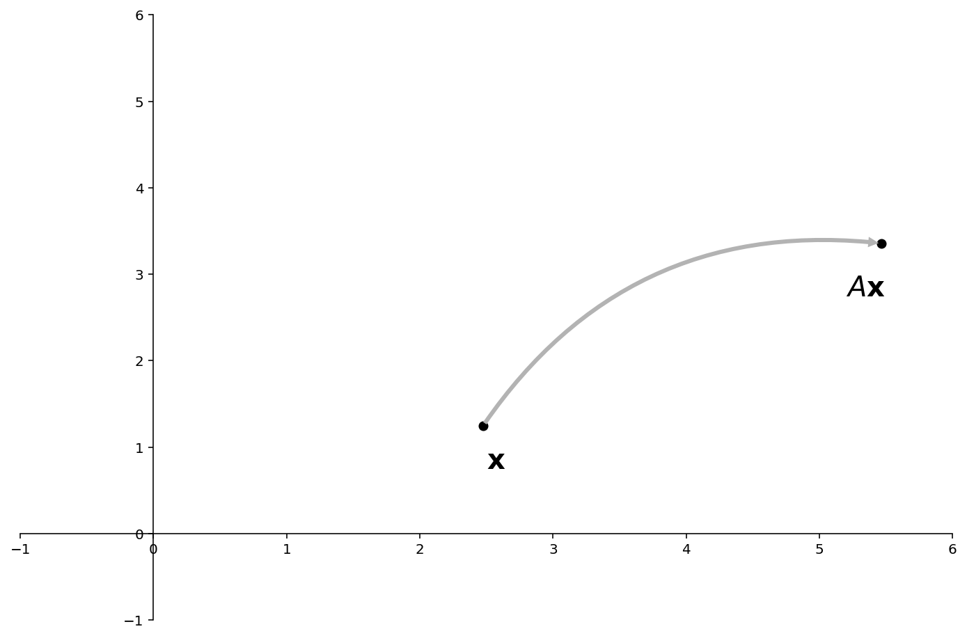
Let’s visualize diagonalization geometrically.

Here is $A$ transforming a point $\mathbf{x} = \begin{bmatrix}2.47\\1.25\end{bmatrix}$.

ax = ut.plotSetup(-1,6,-1,6,size=(12,8))
ut.centerAxes(ax)
v1 = np.array([5.0,1.0])
v1 = v1 / np.sqrt(np.sum(v1*v1))
v2 = np.array([3.0,5.0])
v2 = v2 / np.sqrt(np.sum(v2*v2))
# ut.plotVec(ax,v1,'b')
# ut.plotVec(ax,v2)
# ut.plotLinEqn(-v1[1],v1[0],0,color='b')
# ut.plotLinEqn(-v2[1],v2[0],0,color='r')
# for i in range(-4,8):
#    ut.plotLinEqn(-v1[1],v1[0],i*(v1[0]*v2[1]-v1[1]*v2[0]),format=':',color='b')
#    ut.plotLinEqn(-v2[1],v2[0],i*(v2[0]*v1[1]-v2[1]*v1[0]),format=':',color='r')
p1 = 2*v1+v2
p2 = 4*v1+3*v2
ut.plotVec(ax, p1,'k')
ut.plotVec(ax, p2,'k')
ax.annotate('', xy=(p2[0], p2[1]),  xycoords='data',
                xytext=(p1[0], p1[1]), textcoords='data',
                size=15,
                #bbox=dict(boxstyle="round", fc="0.8"),
                arrowprops={'arrowstyle': 'simple',
                                'fc': '0.7', 
                                'ec': 'none',
                                'connectionstyle' : 'arc3,rad=-0.3'},
                )
ax.text(2.5,0.75,r'${\bf x}$',size=20)
ax.text(5.2,2.75,r'$A{\bf x}$',size=20)
ax.plot(0,0,'');

Now, let’s compute $P^{-1}\mathbf{x}.$

Remember that the columns of $P$ are the eigenvectors of $A$.

So $P^{-1}\mathbf{x}$ is the coordinates of the point $\mathbf{x}$ in the eigenvector basis:

ax = ut.plotSetup(-1,6,-1,6,size=(12,8))
ut.centerAxes(ax)
v1 = np.array([5.0,1.0])
v1 = v1 / np.sqrt(np.sum(v1*v1))
v2 = np.array([3.0,5.0])
v2 = v2 / np.sqrt(np.sum(v2*v2))
ut.plotVec(ax,v1,'b')
ut.plotVec(ax,v2)
ut.plotLinEqn(-v1[1],v1[0],0,color='b')
ut.plotLinEqn(-v2[1],v2[0],0,color='r')
for i in range(-4,8):
    ut.plotLinEqn(-v1[1],v1[0],i*(v1[0]*v2[1]-v1[1]*v2[0]),format=':',color='b')
    ut.plotLinEqn(-v2[1],v2[0],i*(v2[0]*v1[1]-v2[1]*v1[0]),format=':',color='r')
p1 = 2*v1+v2
p2 = 4*v1+3*v2
ut.plotVec(ax, p1,'k')
#ut.plotVec(ax, p2,'k')
#ax.annotate('', xy=(p2[0], p2[1]),  xycoords='data',
#                xytext=(p1[0], p1[1]), textcoords='data',
#                size=15,
                #bbox=dict(boxstyle="round", fc="0.8"),
#                arrowprops={'arrowstyle': 'simple',
#                                'fc': '0.7', 
#                                'ec': 'none',
#                                'connectionstyle' : 'arc3,rad=-0.3'},
#                )
ax.text(2.5,0.75,r'${\bf x}$',size=20)
ax.text(v2[0]-0.15,v2[1]+0.5,r'${\bf p_2}$',size=20)
ax.text(v1[0]-0.15,v1[1]+0.35,r'${\bf p_1}$',size=20)
#ax.text(5.2,2.75,r'$A{\bf x}$',size=16)
ax.plot(0,0,'');

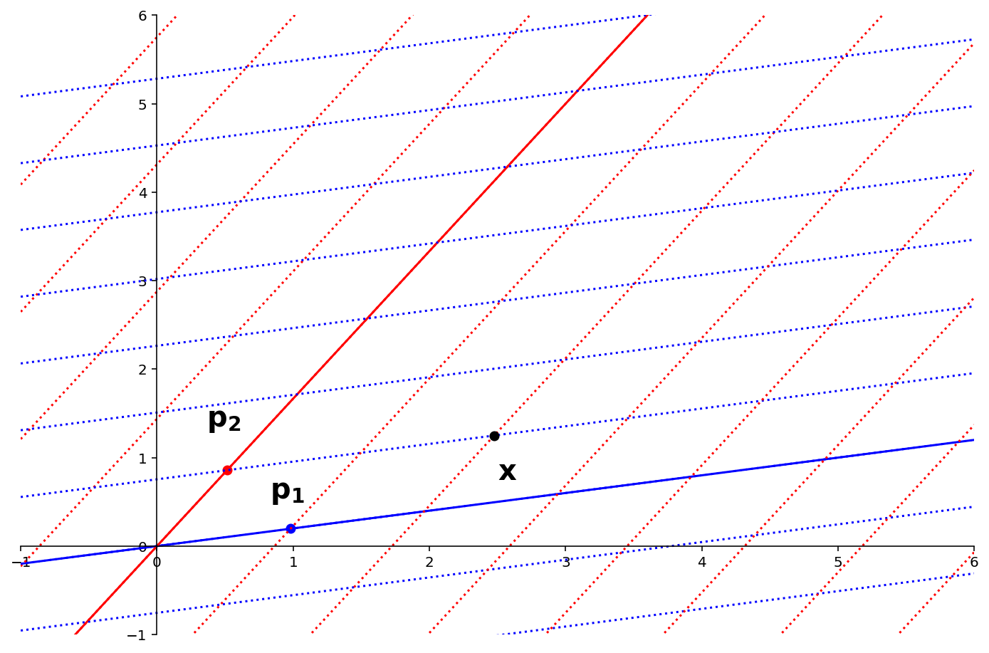
The coordinates of $\mathbf{x}$ in this basis are (2,1).

In other words $P^{-1}\mathbf{x} = \begin{bmatrix}2\\1\end{bmatrix}.$

Now, we compute $DP^{-1}\mathbf{x}.$ Since $D$ is diagonal, this is just scaling each of the $\mathcal{B}$-coordinates.

In this example the eigenvalue corresponding to $\mathbf{p}_1$ is 2, and the eigenvalue corresponding to $\mathbf{p}_2$ is 3.

ax = ut.plotSetup(-1,6,-1,6,size=(12,8))
ut.centerAxes(ax)
v1 = np.array([5.0,1.0])
v1 = v1 / np.sqrt(np.sum(v1*v1))
v2 = np.array([3.0,5.0])
v2 = v2 / np.sqrt(np.sum(v2*v2))
#ut.plotVec(ax,v1,'b')
#ut.plotVec(ax,v2)
ut.plotLinEqn(-v1[1],v1[0],0,color='b')
ut.plotLinEqn(-v2[1],v2[0],0,color='r')
for i in range(-4,8):
    ut.plotLinEqn(-v1[1],v1[0],i*(v1[0]*v2[1]-v1[1]*v2[0]),format=':',color='b')
    ut.plotLinEqn(-v2[1],v2[0],i*(v2[0]*v1[1]-v2[1]*v1[0]),format=':',color='r')
p1 = 2*v1+v2
p2 = 4*v1+3*v2
ut.plotVec(ax, p1,'k')
ut.plotVec(ax, p2,'k')
ax.annotate('', xy=(p2[0], p2[1]),  xycoords='data',
                xytext=(p1[0], p1[1]), textcoords='data',
                size=15,
                #bbox=dict(boxstyle="round", fc="0.8"),
                arrowprops={'arrowstyle': 'simple',
                                'fc': '0.7', 
                                'ec': 'none',
                                'connectionstyle' : 'arc3,rad=-0.3'},
                )
ax.text(2.5,0.75,r'${\bf x}$',size=20)
ax.text(5.2,2.75,r'$A{\bf x}$',size=20)
ax.plot(0,0,'');

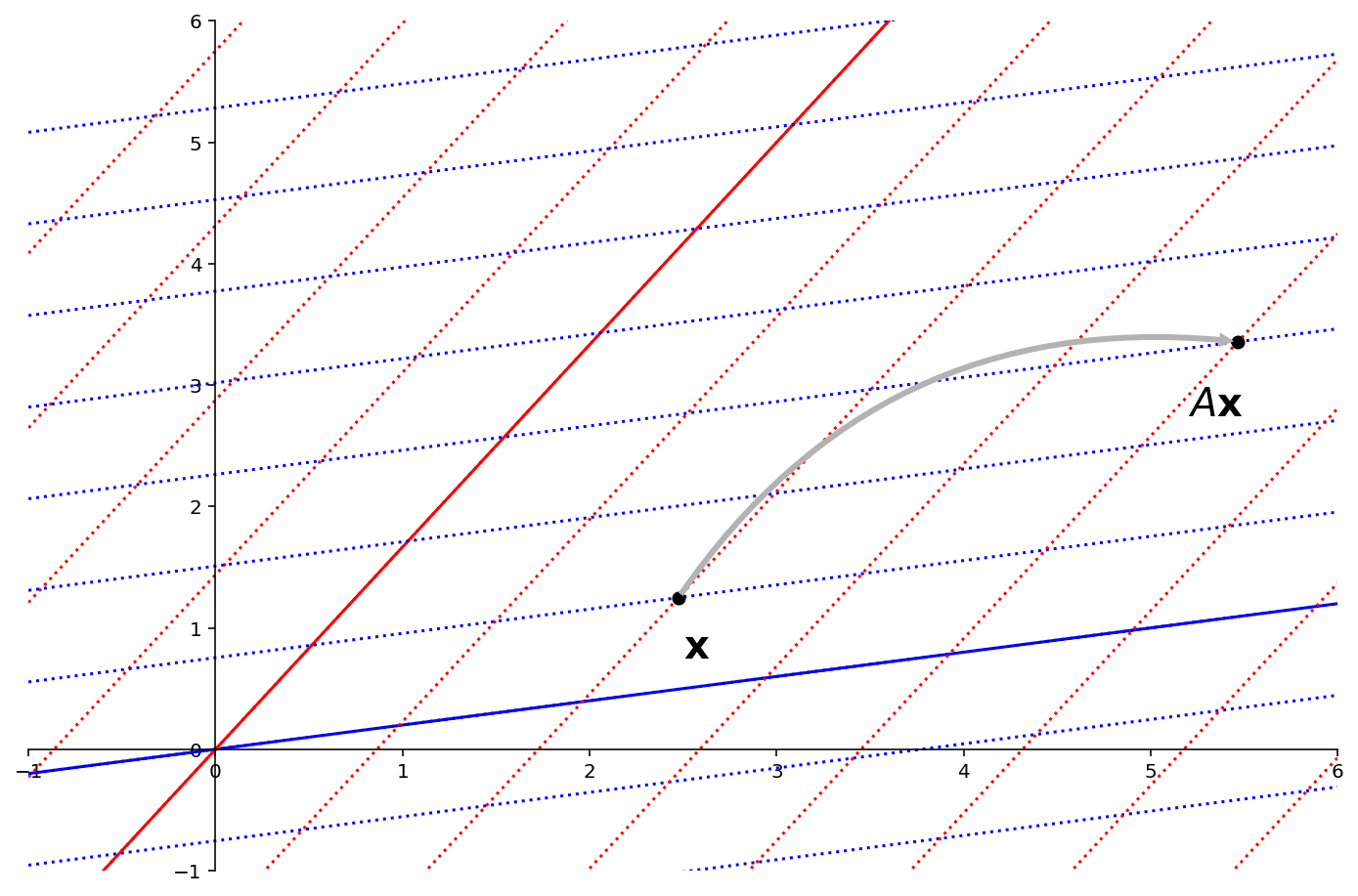
So the coordinates of $A\mathbf{x}$ in the basis $\mathcal{B}$ are

\[\begin{split} \begin{bmatrix}2&0\\0&3\end{bmatrix}\begin{bmatrix}2\\1\end{bmatrix} = \begin{bmatrix}4\\3\end{bmatrix}.\end{split}\]

Now we convert back to the standard basis – that is, we ask which point has coordinates (4,3) in basis $\mathcal{B}.$

We rely on the fact that if $\mathbf{y}$ has coordinates $\mathbf{x}$ in the basis $\mathcal{B}$, then $\mathbf{y} = P\mathbf{x}.$

So

\[\begin{split} A\mathbf{x} = P\begin{bmatrix}4\\3\end{bmatrix}\end{split}\]

\[ = PDP^{-1}\mathbf{x}.\]

ax = ut.plotSetup(-1,6,-1,6,size=(12,8))
ut.centerAxes(ax)
v1 = np.array([5.0,1.0])
v1 = v1 / np.sqrt(np.sum(v1*v1))
v2 = np.array([3.0,5.0])
v2 = v2 / np.sqrt(np.sum(v2*v2))
#ut.plotVec(ax,v1,'b')
#ut.plotVec(ax,v2)
#ut.plotLinEqn(-v1[1],v1[0],0,color='b')
#ut.plotLinEqn(-v2[1],v2[0],0,color='r')
#for i in range(-3,8):
#    ut.plotLinEqn(-v1[1],v1[0],i*(v1[0]*v2[1]-v1[1]*v2[0]),format=':',color='b')
#    ut.plotLinEqn(-v2[1],v2[0],i*(v2[0]*v1[1]-v2[1]*v1[0]),format=':',color='r')
p1 = 2*v1+v2
p2 = 4*v1+3*v2
#ut.plotVec(ax, p1,'k')
ut.plotVec(ax, p2,'k')
#ax.annotate('', xy=(p2[0], p2[1]),  xycoords='data',
#                xytext=(p1[0], p1[1]), textcoords='data',
#                size=15,
#                #bbox=dict(boxstyle="round", fc="0.8"),
#                arrowprops={'arrowstyle': 'simple',
#                                'fc': '0.7', 
#                                'ec': 'none',
#                                'connectionstyle' : 'arc3,rad=-0.3'},
#                )
#ax.text(2.5,0.75,r'${\bf x}$',size=16)
ax.text(5.2,2.75,r'$A{\bf x}$',size=20)
ax.plot(0,0,'');

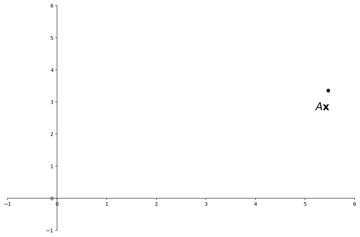
We find that $A\mathbf{x}$ = $PDP^{-1}\mathbf{x} = \begin{bmatrix}5.46\\3.35\end{bmatrix}.$

In conclusion: notice that the transformation $\mathbf{x} \mapsto A\mathbf{x}$ may be a complicated one in which each component of $\mathbf{x}$ affects each component of $A\mathbf{x}$.

However, by changing to the basis defined by the eigenspaces of $A$, the action of $A$ becomes simple to understand.

Diagonalization of $A$ changes to a basis in which the action of $A$ is particularly easy to understand and compute with.

Exposing the Behavior of a Dynamical System¶

At the beginning of the last lecture, we looked at a number of examples of ‘trajectories’ – the behavior of a dynamic system.

Here is a typical example:

sl.display_saved_anim('images/L18-ex1.mp4')

This is the behavior of a dynamical system with matrix $A$:

\[ \mathbf{x}_{k+1} = A\mathbf{x}_k \]

with

\[\begin{split} A = \begin{bmatrix} 0.87142857&0.05714286\\ -0.11428571&1.12857143 \end{bmatrix} \end{split}\]

Looking at $A$ does not give us much insight into why this dynamical system is showing its particular behavior.

Now, let’s diagonalize $A$:

\[ A = PDP^{-1} \]

and we find that:

\[\begin{split} P = \begin{bmatrix} 1&2\\ 4&1 \end{bmatrix}\;\;\;\; \mbox{and}\;\;\;\; D = \begin{bmatrix} 1.1 & 0\\ 0 & 0.9 \end{bmatrix} \end{split}\]

The columns of $P$ are eigenvectors of $A$ that correspond to the eigenvalues in $D$.

So the eigenspace corresponding to $\lambda_1 = 1.1$ is Span$\left\{\begin{bmatrix}1\\4\end{bmatrix}\right\}$,

and the eigenspace corresponding to $\lambda_2 = 0.9$ is Span$\left\{\begin{bmatrix}2\\1\end{bmatrix}\right\}$.

Let’s look at these eigenspaces:

display(Image('images/L18-ex1-static.png'))

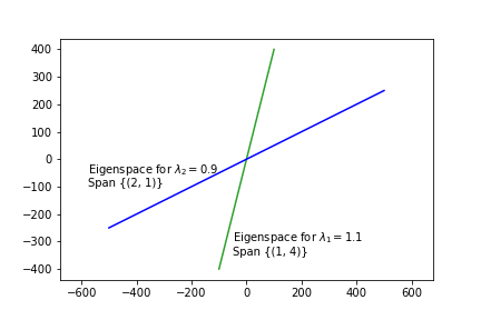
Now, the behavior of this dynamical system becomes much clearer!

sl.display_saved_anim('images/L18-ex2.mp4')

The initial point has a large component in the blue eigenspace, and a small component in the green eigenspace.

As the system evolves, the blue component shrinks by a factor of 0.9 on each step,

and the green component increases by a factor of 1.1 on each step.

Which allows us to understand very clearly why the dynamical system shows the behavior it does!

Linear Algebra, Geometry, and Computation

Diagonalization¶

Powers of a Diagonal Matrix¶

Extending to a general matrix \(A\)¶

Diagonalization Requires Eigenvectors and Eigenvalues¶

Diagonalizing a Matrix¶

Four Steps to Diagonalization¶

Step 1: Find the eigenvalues of \(A\).¶

Step 2: Find three linearly independent eigenvectors of \(A\).¶

Step 3: Construct \(P\) from the vectors in Step 2.¶

Step 4: Construct \(D\) from the corresponding eigenvalues.¶

When Diagonalization Fails¶

An Important Case¶

Diagonalization as a Change of Basis¶

Interpreting Diagonalization Geometrically¶

Exposing the Behavior of a Dynamical System¶